Download
1 / 43
430 likes | 618 Vues
MODELING COMMODITY PRICES WITH DYNAMIC CONDITIONAL BETA. ROBERT ENGLE DIRECTOR: VOLATILITY INSTITUTE AT NYU STERN RECENT ADVANCES IN COMMODITY MARKETS QUEEN MARY, NOV,8,2013. VOLATIliTY AND ECONOMIC DECISIONS. Asset prices change over time as new information becomes available.

E N D
MODELING COMMODITY PRICES WITH DYNAMIC CONDITIONAL BETA ROBERT ENGLE DIRECTOR: VOLATILITY INSTITUTE AT NYU STERN RECENT ADVANCES IN COMMODITY MARKETS QUEEN MARY, NOV,8,2013
VOLATIliTY AND ECONOMIC DECISIONS • Asset prices change over time as new information becomes available. • Both public and private information will move asset prices through trades. • Volatility is therefore a measure of the information flow. • Volatility is important for many economic decisions such as portfolio construction on the demand side and plant and equipment investments on the supply side. NYU VOLATILITY INSTITUTE
RISK • Investors with short time horizons will be interested in short term volatility and its implications for the risk of portfolios of assets. • Investors with long horizons such as commodity suppliers will be interested in much longer horizon measures of risk. • The difference between short term risk and long term risk is an additional risk – “The risk that the risk will change” NYU VOLATILITY INSTITUTE
commodities • The commodity market has moved swiftly from a marketplace linking suppliers and end-users to a market which also includes a full range of investors who are speculating, hedging and taking complex positions. • What are the statistical consequences? • Commodity producers must choose investments based on long run measures of risk and reward. • In this paper I will try to assess the long run risk in these markets. NYU VOLATILITY INSTITUTE
The s&pgsci database • The most widely used set of commodities prices is the GSCI data base which was originally constructed by Goldman Sachs and is now managed by Standard and Poors. • I will use their approximation to spot commodity price returns which is generally the daily movement in the price of near term futures. The index and its components are designed to be investible. NYU VOLATILITY INSTITUTE
volatility • Using daily data from 1996 to July, 2012, annualized measures of means and volatilities are constructed for 21 different commodities. These are roughly divided into agricultural, industrial, precious metals and energy products. NYU VOLATILITY INSTITUTE
Tail risk measure:ANNUAL 1% VAR? • What annual return from today will be worse than the actual return 99 out of 100 times? • What is the 1% quantile for the annual percentage change in the price of an asset? • Assuming constant volatility and a normal distribution, it just depends upon the volatility. Here is the result. Here also is the actual 1% quantile of overlapping annual returns for each series since 1996. NYU VOLATILITY INSTITUTE
A 1% chance NYU VOLATILITY INSTITUTE
1% annual vAr and 1% realized quantile(of all 252 day returns, what is 1% quantile) NYU VOLATILITY INSTITUTE
But are these volatiltiies constant? • Like most financial assets, volatilities change over time. • Vlab.stern.nyu.edu is a web site at the Volatility Institute that estimates and updates volatility forecasts every day for several thousand assets. It includes these and other GSCI assets. NYU VOLATILITY INSTITUTE
Volatility of copper, nickel, aluminum NOVEMBER 7, 2013 NYU VOLATILITY INSTITUTE
GOLD, SILVER, PLATINUM NYU VOLATILITY INSTITUTE
The risk that the risk will change • We would like a forward looking measure of VaR that takes into account the possibility that the risk will change and that the shocks will not be normal. • LRRISK calculated in VLAB does this computation every day. • Using an estimated volatility model and the empirical distribution of shocks, it simulates 10,000 sample paths of commodity prices. The 1% and 5% quantiles at both a month and a year are reported. NYU VOLATILITY INSTITUTE
COPPER:ONE YEAR AHEAD 1% VAR NYU VOLATILITY INSTITUTE
GOLD: ANNUAL 1% VAR NYU VOLATILITY INSTITUTE
Relation to macroeconomic factors • Some commodities are more closely connected to the global economy and consequently, they will find their long run VaR depends upon the probability of global decline. • We can ask a related question, how much will commodity prices fall if the macroeconomy falls dramtically? • Or, how much will commodity prices fall if stock prices fall. NYU VOLATILITY INSTITUTE
WHAt is the consequence? NYU VOLATILITY INSTITUTE
Commodity beta • Estimate the model • Where y is the logarithmic return on a commodity price and x is the logarithmic return on an equity index. • If beta is time invariant and epsilon has conditional mean zero, then MES and LRMES can be computed from the Expected Shortfall of x. • But is beta really constant? • Is epsilon serially uncorrelated? NYU VOLATILITY INSTITUTE
DYNAMIC CONDITIONAL BETA • This is a new method for estimating betas that are not constant over time and is particularly useful for financial data. See Engle(2012). • It has been used to determine the expected capital that a financial institution will need to raise if there is another financial crisis and here we will use this to estimate the fall in commodity prices if there is another global financial crisis. • It has also been used in Bali and Engle(2010,2012) to test the CAPM and ICAPM. NYU VOLATILITY INSTITUTE
MODELLING TIME VARYING BETA • ROLLING REGRESSION • INTERACTING VARIABLES WITH TRENDS, SPLINES OR OTHER OBSERVABLES • TIME VARYING PARAMETER MODELS BASED ON KALMAN FILTER • STRUCTURAL BREAK AND REGIME SWITCHING MODELS • EACH OF THESE SPECIFIES CLASSES OF PARAMETER EVOLUTION THAT MAY NOT BE CONSISTENT WITH ECONOMIC THINKING OR DATA.
THE BASIC IDEA • IF is a collection of k+1 random variables that are distributed as • Then • Hence:
implications • We require an estimate of the conditional covariance matrix and possibly the conditional means in order to express the betas. • In regressions such as one factor or multi-factor beta models or money manager style models or risk factor models, the means are insignificant and the covariances are important and can be easily estimated. • In one factor models this has been used since Bollerslev, Engle and Wooldridge(1988) as
HOW TO ESTIMATE H • Econometricians have developed a wide range of approaches to estimating large covariance matrices. These include • Multivariate GARCH models such as VEC and BEKK • Constant Conditional Correlation models • Dynamic Conditional Correlation models • Dynamic Equicorrelation models • Multivariate Stochastic Volatility Models • Many many more • Exponential Smoothing with prespecified smoothing parameter.
Is beta constant? • For none of these methods will beta appear constant. • In the one regressor case this requires the ratio of to be constant. • This is a non-nested hypothesis • More precisely it is a partially nested model. The point at which these models are nested is when there is no heteroskedasticity and hence they are identical. Pretest for heteroskedasticity.
Artificial nesting • Create a model that nests both hypotheses. • Test the nesting parameters • Four possible outcomes • Reject f • Reject g • Reject both • Reject neither
ARTIFICIAL NESTING • Consider the model: • If , the parameters are constant • If , the parameters are time varying. • If both are non-zero, the nested model may be entertained. • Notice that with several regressors there are many possible outcomes. • SUGGESTION: Nested Model is the MODEL
Application to commodities • Estimate regression of commodity returns on SP 500 returns. There is substantial heteroskedasticity in residuals. • Sample is daily 1996 – July 2012 • Do Rolling Regression Model • Estimate beta from sample of t-n-1 to t-1 • Using this estimated beta calculate residual at t • Compute sum of squared residuals for all t • Minimize over n • Note: no correction for heteroskedasticity NYU VOLATILITY INSTITUTE
Dcb model for aluminum NYU VOLATILITY INSTITUTE
Dcc parameters for aluminum • The daily decay rate of the correlations is .998. This is very slow moving but is indeed mean reverting. It has a half life of about one and a half years. • The GJR-GARCH model for aluminum has a persistence of .993 for a half life of about 100 days. • The GJR-GARCH model for SP_500 is highly asymmetric and has a persistence of .9868 for a half life of 50 days. • The beta is the correlation times the ratio of these two volatilities, it is not clear how persistent it really is. NYU VOLATILITY INSTITUTE
Testing for constancy NYU VOLATILITY INSTITUTE
results • DCB has smaller (better) SIC for all 21 commodities. • This is not the case for other data sets. For FF data on industry sectors, about half favor constant beta and half favor time variation. • Two of the constant betas are insignificant at 5% value. • One of the dynamic betas fails to have a t-stat greater than two. NYU VOLATILITY INSTITUTE
results • Set s=t • Grid search yields • Schwarz Criterion STR 3.220 • Schwarz Criterion Constant beta 3.247 • Schwarz Criterion DCB 3.216 NYU VOLATILITY INSTITUTE
SMOOTH TRANSITION MODEL NYU VOLATILITY INSTITUTE
Out of sample results • Are these changes in beta permanent? • Will resources become decoupled from broad equity indices? • Today the stock market is rising while commodities are tanking. • STR model cannot adjust to a return very quickly because it is difficult to see regime changes until there is sufficient data after the change. • What does DCB show? NYU VOLATILITY INSTITUTE
Vlab COMMODITY CORRELATIONS NYU VOLATILITY INSTITUTE
Gold, platinum, silver correlations NYU VOLATILITY INSTITUTE
Brent, gasoline, heating oil NYU VOLATILITY INSTITUTE
Grains, sugar, cattle, hogs NYU VOLATILITY INSTITUTE
COMMODITY CORELLATION FACTORS (first two eigenvalues) NYU VOLATILITY INSTITUTE
Conclusions and findings • The one year VaR changes over time as the volatility changes. • The betas on equity markets have risen dramatically since the financial crisis. • The value of commodities for diversification has been reduced but not eliminated. • There is evidence post sample that correlations for some commodities are mean reverting while others are not. NYU VOLATILITY INSTITUTE