Download
1 / 19
270 likes | 641 Vues
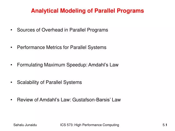
Analytical Modeling of Parallel Programs. Sources of Overhead in Parallel Programs Performance Metrics for Parallel Systems Formulating Maximum Speedup: Amdahl’s Law Scalability of Parallel Systems Review of Amdahl’s Law: Gustafson-Barsis’ Law. Analytical Modeling - Basics.

E N D
Analytical Modeling of Parallel Programs • Sources of Overhead in Parallel Programs • Performance Metrics for Parallel Systems • Formulating Maximum Speedup: Amdahl’s Law • Scalability of Parallel Systems • Review of Amdahl’s Law: Gustafson-Barsis’ Law
Analytical Modeling - Basics • A sequential algorithm is evaluated by its runtime (in general, asymptotic runtime as a function of input size). • The asymptotic runtime of a sequential program is identical on any serial platform. • On the other hand, the parallel runtime of a program depends on • the input size, • the number of processors, and • the communication parameters of the machine. • An algorithm must therefore be analyzed in the context of the underlying platform. • A parallel system is a combination of a parallel algorithm and an underlying platform.
Sources of Overhead in Parallel Programs • If I use n processors to run my program, would it run n times faster? • Overheads! • Interprocessor Communication & Interactions • Usually the most significant source of overhead • Idling • Load imbalance, Synchronization, Serial components • Excess Computation • Sub-optimal serial algorithm • More aggregate computations • Goal is to minimize these overheads!
Performance Metrics for Parallel Programs • Why analyze the performance of parallel programs? • Determine the best algorithm • Examine the benefit of parallelism • A number of metrics have been used based on the desired outcome of performance analysis: • Execution time • Total parallel overhead • Speedup • Efficiency • Cost
Performance Metrics for Parallel Programs • Parallel Execution Time • Time spent to solve a problem on p processors. • Tp • Total Overhead Function • To = pTp – Ts • Speedup • S = Ts/Tp • Can we have superlinear speedup? • exploratory computations, hardware features • Efficiency • E = S/p • Cost • pTp(processor-time product)
Performance Metrics: Example on Speedup • What is the benefit from parallelism? • Consider the problem of adding n numbers by using n processing elements. • If n is a power of two, we can perform this operation in log n steps by propagating partial sums up a logical binary tree of processors. • If an addition takes constant time, say, tcand communication of a single word takes time ts + tw, the parallel time is TP = Θ (log n) • We know that TS = Θ (n) • Speedup S is given by S = Θ (n / log n)
Performance Metrics: Speedup Bounds • For computing speedup, the best sequential program is taken as the baseline. • There may be different sequential algorithms with different asymptotic runtimes for a given problem • Speedup can be as low as 0 (the parallel program never terminates). • Speedup, in theory, should be upper bounded by p. • In practice, a speedup greater than p is possible. • This is known as superlinear speedup • Superlinear speedup can result • when a serial algorithm does more computations than its parallel formulation • due to hardware features that put the serial implementation at a disadvantage • Note that superlinear speed happens only if each processing element spends less than time TS/p solving the problem.
Performance Metrics: Superlinear Speedups • Superlinearity effect due to exploratory decomposition
Cost of a Parallel System • As shown earlier, Cost is the product of parallel runtime and the number of processing elements used (pTP). • Cost reflects the sum of the time that each processing element spends solving the problem. • A parallel system is said to be cost-optimal if the cost of solving a problem on a parallel computer is asymptotically identical to serial cost. • Since E = TS / p TP, for cost optimal systems, E = O(1). • Cost is sometimes referred to as work or processor-time product. • The problem of adding n numbers on n processors is not cost-optimal.
Formulating Maximum Speedup • Assume an algorithm has some sequential parts that are only executed on one processor. • Assume the fraction of the computation that cannot be divided into concurrent tasks is f. • Assume no overhead incurs when the computation is divided into concurrent parts. • The time to perform the computation with pprocessors is: • Hence, the speedup factor is (Amdahl’s Law):
Speedup against number of processors • From the preceding formulation, f has to be a small fraction of the overall computation if significant increase in speedup is to occur • Even with infinite number of processors, maximum speedup limited to 1/f: • Example: With only 5% of computation being serial, maximum speedup is 20, irrespective of number of processors. • Amdahl used this argument to promote single processor machines
Scalability • Speedup and efficiency are relative terms. They depend on • Number of processors • Problem size • The algorithm used • For example, efficiency of a parallel program often decreases as the number of processors increases • Similarly, a parallel program may be quite efficient for solving large problems, but not for solving small problems • A parallel program is said to scale if its efficiency is constant for a broad range of number of processors and problem sizes • Finally, speedup and efficiency depend on the algorithm used. • A parallel program might be efficient relative to one sequential algorithm but not relative to a different sequential algorithm
Gustafson’s Law • Presented an argument based upon scalability concepts. • To show that Amdahl’s law was not as significant as first supposed in limiting the potential speedup. • Observation: In practice a larger multiprocessor usually allows a larger size of the problem to be undertaken in a reasonable execution time. • Hence, the problem size is not independent of the number of processors. • Rather than assume the problem size is fixed, we should assume that the parallel execution time is fixed. • Using the parallel constant execution time constraint, the resulting speedup factor will be numerically different from Amdahl’s speedup factor and is called a scaled speedup factor
Formulating Gustafson’s Law • Assuming the parallel execution time, Tp, is normalized to unity: • Assuming that in the serial execution time, Ts, below, fTs is a constant, • Then the scaled speedup factor (Gustafson’s Law) is: