Download
1 / 21
220 likes | 521 Vues
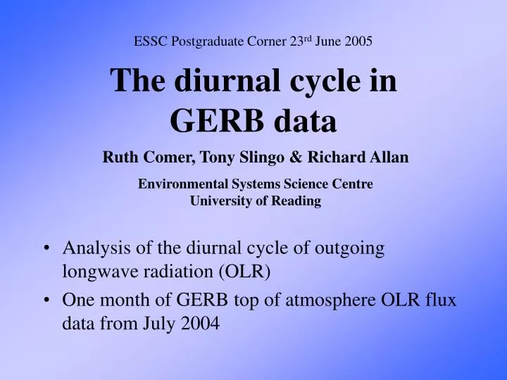
ESSC Postgraduate Corner 23 rd June 2005. The diurnal cycle in GERB data. Analysis of the diurnal cycle of outgoing longwave radiation (OLR) One month of GERB top of atmosphere OLR flux data from July 2004. Ruth Comer, Tony Slingo & Richard Allan

E N D
ESSC Postgraduate Corner 23rd June 2005 The diurnal cycle in GERB data • Analysis of the diurnal cycle of outgoing longwave radiation (OLR) • One month of GERB top of atmosphere OLR flux data from July 2004 Ruth Comer, Tony Slingo & Richard Allan Environmental Systems Science CentreUniversity of Reading
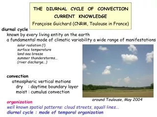
Why study the diurnal cycle? • The diurnal cycle represents one of the most significant modes of atmospheric variability • OLR provides information about surface heating response and cloud variation • OLR is a major contributor to the Earth’s Radiation Budget • Small diurnal variations may have implications for long term climate change
Background This type of diurnal cycle study has a long history. Recent publications include: • G Yang & J Slingo 2000 • Fourier analysis in CLAUS Data • L Smith & D Rutan 2002 • EOF analysis in ERBS Data • B Tian, B Soden & X Wu 2004 • Time series and Fourier analysis comparing Satellite observations with GCM
GERB • Geostationary Earth Radiation Budget instrument on-board Meteosat-8 • First to measure broadband OLR from geostationary orbit – high temporal resolution • Location above Africa makes GERB ideal for diurnal cycle study • OLR fluxes calculated from total and shortwave • Processed onto regular 0.556lat × 0.833lon grid
Processing • One Month of GERB OLR Barg data from July 2004 • Simple time series mean plots and histograms • Average Month onto single day • Mean plots/histograms • EOF Analysis • Fourier Analysis
y j i x What is EOF analysis? • Method for looking at time- and space-dependent variables • Finds an orthogonal basis to efficiently describe the variation in a data set • Empirical Orthogonal Functions (EOFs) • Describe variation of data over area • Principal Components (PCs) • Describe variation of data with time
space time The maths bit Consider the data in matrix form with the overall mean at each location removed EOF analysis finds a vector a such that the variance of c=Xa is maximised (Each entry in a corresponds to a location in our physical domain Each entry in c corresponds to a time-step)
What does this mean? To illustrate, suppose we choose corresponding to a single point in the domain Then Gives a mean diurnal cycle at that point. But we want to represent the whole domain
What does this mean? We could represent each location equally i.e. Then Mean diurnal cycle over the whole domain The first EOF is a with more weighting given to locations with more variation…
We do this by giving greater weighting to the areas that vary the most EOF1= a What does this mean? PC1= c To understand the variation of the data set we want to give c maximum variance
First EOF & PC PC1 describes 77.6% of the total variance • Strong signal over deserts suggests surface heating response • Note some small negative signals around African coast
Contribution from PC1 Contribution from PC1 Mean curve Comparison of PC1 with Sahara mean EOFs/PCs do not necessarily describe physical modes in the data, however
Subsequent EOFs To find the second EOF and PC we remove the contribution of the first from our data and repeat the process. i.e. (xpn is data point at location p, time-step n) The number of EOFs required to describe the entire variation of the data is less than or equal to the number of time-steps (cf Fourier analysis) We can reconstruct the original data from the EOFs:
Convective cloud Stratus Second EOF & PC PC2 describes 12.8% of total variance Hence first 2 PCs describe 90.4% Provides modification to PC1 for cloud
Contribution from PC2 Contribution from PC2 Mean curve Southern Atlantic
Atlas Mountains Hoggar Tibesti Marra Plateau Ethiopian & Yemeni highlands Topography visible in second EOF
Cloudy Mean curve Mean curve Mean curve Contribution from PC1 Contribution from PC1 Combined contributions from PCs 1&2 TRMM shows maximum precip here (Nesbitt & Zipser 2002) Clear sky Central Africa
Mean curve Contribution from PC1 Contribution from first 2 PCs Contribution from first 3 PCs EOF3 PC3 Gulf of Guinea
0 6 12 18 24 Gulf of Guinea Desbois et al (1988) suggest diurnal cycle of cloud here is forced by land-sea breeze effects
Conclusions • EOF Analysis on GERB OLR data appears to pick up surface heating and cloud responses well (with certain exceptions) • PC1 describes surface response to heating • PC2 describes cloud development • Convective • Stratus • Shows significance of topography
Future Work • Comparison of GERB with other data • ?TRMM • SEVIRI • RADAGAST • Investigation of models • Met Office NWP model • HiGEM • Cloud resolving models