Download
1 / 18
190 likes | 351 Vues
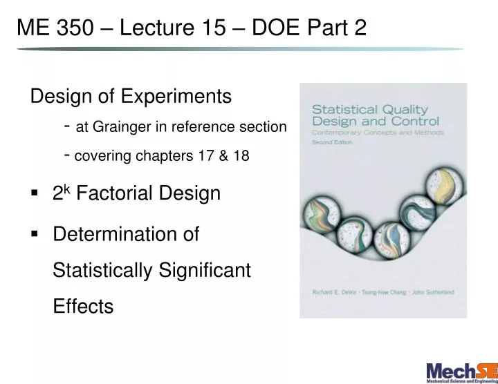
ME 350 – Lecture 15 – DOE Part 2. Design of Experiments - at Grainger in reference section - covering chapters 17 & 18 2 k Factorial Design Determination of Statistically Significant Effects. 2 3 Factorial Design Example. Study on the alertness of students in the morning: Variables

E N D
ME 350 – Lecture 15 – DOE Part 2 Design of Experiments - at Grainger in reference section - covering chapters 17 & 18 • 2k Factorial Design • Determination of Statistically Significant Effects
23 Factorial Design Example Study on the alertness of students in the morning: • Variables • Design Matrix
75 (+,+,+) 59 (-,+,+) 4 Food, X3 8 62 (+,-,+) 43 (-,-,+) 6 2 CoffeeX2 3 89 (+,+,-) 7 Sleep, X1 1 56 (-,-,-) 72 (+,-,-) 5 Effect of Variables? 68 (-,+,-)
Use Matrix Algebra to Solve: • Eliminating the “insignificant effects” yields the final equation:
Effect of Variables • The sign of the effect indicates its direction – whether the response • The magnitude indicates the effect: • If “compound” effects are negligible then the two effects are said to be: E1 = 18 E3 = -11.5
Determining Statistically Significant Effects Two methods: • If test experiments are duplicated (at least once) then result variance can be calculated. If the Effect value is outside of the system variability, then it is significant. • Effects can be plotted graphically. If all effects are insignificant then they will form what distribution around zero? Variable effects that fall outside this distribution are significant.
1. Statistical Variance Determination • This approach assumes the amount of variance in an observation is the for all observations. • Thus the variance of the system is:
1. Statistical Variance Determination - Ex • Remember our Alertness Experiment:
1. Statistical Variance Determination - Ex • To determine if an effect is statistically significant: • Determine the System Standard Deviation (as done previously) • Determine the 95% confidence interval: • If effect is outside of this range, then it is
1. Statistical Variance Determination - Ex • If the effect is “outside” ±2σ, then the effect is significant Determine statistically significant effects • Significant effects:
2. Gaussian Analysis of “Noise?” Ave. measurement is 9.27, with some variability; there are measurements less than 9.2, but not very often. The farther from the mean the less likely a reading will occur. Norm. Prob. Plot is a straight line for noise. Non-significant effects will be like “noise” – lying along a straight line roughly centered around zero on a Norm. Prob. graph. *http://www.itl.nist.gov/div898/handbook/pri/pri.htm
2. Cumulative Probability Graph • A 2k factorial experiment was run with the following “Effects” calculated: -0.15, -0.45, 0.2, 0, 0.85, 0.45, -0.9 • Is the 0.85 significant? How about the -0.9? • To determine the significant effects, put them first in ascending order: The lowest value should represent the lower , or the 0 to14.29% range (on a graph placed midway at 7.14%). The next value represents the 14.3 to 28.5% range. Cumulative Probability: X position determined by excel formula: = NORMSINV()
2. Graphical Analysis • Since all the effects end up on a straight line around zero (i.e. 50%), their values are due to “noise” and are not significant in value. • Instead of creating Cumulative Probability Plots, is there an easier way? Equidistant plots work well?
2. Graphical Approach Example • Assume the Effect values were: 8, 1.5, -0.5, 6, -2, 10, 0.5 Which are insignificant?
2. Equidistant Graph? • Which are significant? • First find (0,0) point – draw flattest line (smallest effects) • Points not on/near line are:
Original Example • Part weight characteristic equation: • Variability analysis:
Fractional Factorial Design • Assuming there are 7 variables to test, then 27 (128) experiments will need to be run • Fractional Factorial designs can accomplish this with only 8 tests: