Download
1 / 14
150 likes | 304 Vues
Bayesian statistics. 3. Bayesian statistics. Probability theory and statistics are important in genomics: - Evolution itself is stochastic in nature - Large amounts of data make statistical approaches powerful - Significance: unlikely things do happen in large genomes

E N D
3. Bayesian statistics Probability theory and statistics are important in genomics: - Evolution itself is stochastic in nature - Large amounts of data make statistical approaches powerful - Significance: unlikely things do happen in large genomes Two schools of thought: Frequentists and Bayesians. In both cases, the concept of “probability” is used. It is mathematically formalized in the same way, but has a (slightly) different interpretation. Jerzy Neyman (1894 – 1981) Ronald A Fisher (1890-1962) Rev. Thomas Bayes (1702-1761) Confidence interval Max Likelihood; ANOVA Bayes’ Formula
Axioms of probability theory Basic concepts are: * Sample spaceΩ is the set of all possible outcomes (examples: {head,tails}; all possible trajectories DJ(t) of the Dow-Jones index over time) * EventsEare subsets ofΩ (examples: {head}; Dow-Jones = 10000 at January 1st = { DJ(t) | DJ(Jan 1st) = 10000 }.) * Probability measureP, assigns a real number to subsets E, with properties: - P(Ω) = 1 - P() = 0 - P(A B) = P(A) + P(B) if A,B are disjunct (do not share elements) (Technical note: not all subsets E may be allowed; in the case that Ω is very large, e.g. all real numbers, or functions, it turns out to be necessary to restrict yourself to “well behaved” subsets, known as “measurable” sets.) (Another technical note: In the case that Ωis not a discrete set, P is a probability density, P(E) dE, defined with respect to another measure dE)
Bayesian vs. Frequentist Frequentist: • E models actual outcomes ofrepeatable experiments • P(E) models their frequency of occurrence • Adequacy of P assessed by hypothesis testing • When the model P depends on a parameter , the most likely value is preferred Bayesian: • E models both actual outcomes and underlying hypotheses or parameters • For a model P, is considered a random variable rather than a fixed parameter • The interpretation of P(E) is different for the two “components” of E: • Observables: the frequency of the actual occurrences as before • Hypotheses / parameters: belief in (plausibility of) truth or value. • Adequacy of a hypothesis H is tested by computing its posterior probability • Bayesian approaches include prior probabilities: beliefs before seeing any data Difference between the two approaches lies mostly in the interpretation. Many researchers use both. Bayesian approaches are useful with limited amounts of data, as prior information is included. With lots of data, the prior does not influence the result, and the two approaches give the same answers.
Bayesian vs. Frequentist: inference Frequentist: • Parameters of the model are considered to have a single true (but unknown) value. P(E) models the parameter-dependent frequency-of-occurrence of E. • As a function of (rather than of E), P(E) is called the likelihood of E. • Parameters are estimated by maximizing the likelihood for a given event E. Example: Drawing red and black balls from an urn (with replacement). Urn contains a proportion of red balls. Draw N balls. E = {n red, m=N-n black balls drawn}. This has a maximum for = n / (n+m). This seems reasonable if n and m are large. However, suppose you’ve been asked to estimate the probability that the next ball is red. If n=1, m=0, the maximum likelihood estimate for clearly is not a reasonable estimate for this probability, if it is interpreted as your belief in the prediction. This interpretation is quite natural, for instance it is the way you interpret the statement “there is a 70% probability that it will rain tomorrow”.
Bayesian vs. Frequentist: inference Bayesian: • Parameters of the model are considered to be unknown, but not all parameter values are (necessarily) equally likely a priori • is part of the sample space; the model specifies the joint probabilityP(E, ). • The posterior P(|E) is computed by Bayes’ rule: P(|E) = P(E|) P() / P(E). Here, P() is the prior probability of the various values that can take. • Parameter are estimated from the posteriorP(|E)for. Example: Drawing red and black balls from an urn (with replacement). Urn contains a proportion of red balls. Draw N balls. E = {n red, m=N-n black balls drawn}. Multiply with a uniform prior P() = 1d: Calculate P(E):(n+m+1 possibilities) Dividing (*) by P(E) gives posterior. Posterior mean value of : (n+1) / (n+m+2) (Posterior averaging: typical Bayesian approach). Maximum of posterior: n / (n+m) (Maximum a-posteriori [MAP] estimate) MAP = MLE when uniform priors are used
Bayes’ Rule and conditional probabilities Straightforwardly, P(E) is the probability of the event E, compared to the “universe” Ω of possibilities. Suppose you know that the outcome (an element of E) will be from a set C Ω. Other than that, the situation is the same. Outcomes that are not in C are simply excluded. The probability of event E in this case is called the conditional probability ofEgiven (or conditional on)C, symbolically P(E | C) Note that not all outcomes specified by E are necessarily in C. They may even be disjunct (non-overlapping), in which case the probability of E given C (or: conditional on C) is 0. Example: there is a certain probability, on any given day, that the sun shines. However, if we know that it was sunny yesterday, the probability is higher. The formula for the conditional probability is Here, P(E,θ) = P(Eθ) is the probability that both E and θ happened (i.e. the outcome is in both E and θ).
Conditional Probabilities – Monty Hall problem There are 3 doors. Behind one door is a prize; there is nothing behind the other two. You pick one of the doors – but Money doesn’t open it yet. To show you how lucky you were, Monty then opens one of the doors you didn’t choose - without the prize. Which of the two unopened doors is more likely to hide the prize?
Bayes’ Rule and conditional probabilities Bayes’ Rule is the formula that tells you how to convert a conditional probability of (say) data conditional on (say) an unknown parameter, into the probability of that parameter conditional on the data. The factor P(E| θ) is called the likelihood (when considered as a function of θ). The probability P(E) is the marginal probability of the event E; it acts as a normalizing constant. Sometimes this is hard to compute; luckily, for many applications you can do without. The factor P(θ) is the prior probability of θ(since it does not take the data E into account) The left-hand side P(θ|E) is the posterior of θ. Bayes’ rule can be derived from the definition of conditional probability, , which is all you need to remember.
Bayes’ Rule and conditional probabilities Let the random variable θdenote where the prize is (1,2,3) Initially there is nothing to distinguish the doors – so without loss of generality (W.L.O.G), say you chose door 1. Again W.L.O.G, suppose Monty opened door 2 to reveal no prize. Let E denote this event. Conditional probabilities of E given the 3 possibilities for θare: P( E| θ=1 ) = 1/2 P( E| θ=2 ) = 0 P( E| θ=3 ) = 1 We have no reason to favour any of the 3 doors, so the prior for θis uniform, 1/3 for all three possibilities. The probability of E is intuitively ½ (Monty could only choose from 2 doors), but we do not need intuition: P( E ) = θP(E,θ) = θP(E | θ) P(θ) = 1/2*1/3 + 1*1/3 = ½ The posterior probability of θ=3 is now P(θ=3 | E) = P(E | θ=3) P(θ=3) / P( E ) = (1 * 1/3) / ½ = 2/3
Equilibrium, reversibility, and MCMC Very often, you have some complicated model P(D, θ) describing the joint distribution of data D and parameters θ, and you’re interested in the posterior P(θ|D) for some observation D. you often want to compute the average of some function over the posterior. This is often impossible to calculate directly. The trick with MCMC is to construct a Markov chain whose equilibrium distribution is precisely P(θ|D). Now, computing the equilibrium distribution as the left eigenvector of 0 is impossible for Markov model with many states if there is no special structure. So it is very hard to construct a Markov chain with a desired equilibrium distribution. For reversible models however, the equilibrium distribution is easy to determine. Conversely, you can design Markov models to have any particular equilibrium distribution, as long as the model is reversible.
vx Rxy x y vy Ryx Equilibrium, reversibility, and MCMC Equilibrium distribution: vR = 0 or x vx Rxy = 0 for all y. Reversibility:vx Rxy = vy Ryxfor all x and y. Reversibility (of v and R) implies equilibrium: x vx Rxy = x vy Ryx = vy x Ryx = 0 So reversibility (for v) is a stronger condition than being an equilibrium distribution. Intuitively, it says that the total “flow” across any arrow of the Markov chain is 0: there are no “loops”. It is called “reversible” because if this condition holds, you cannot tell the direction of time by looking at a system (in equilibrium). The laws of physics have this property (at thermal equilibrium).
x y Metropolis-Hastings algorithm Now suppose you want a Markov chain whose equilibrium is vx = P(x). Here is the recipe: A. Decide between which pairs of states x,y you will allow transitions. This must be (i) symmetric (if xy then yx), (ii) all states must be reachable from any other, and (iii) the network must be “aperiodic”. B. Decide on a “proposal distribution” Q(y|x), which proposes transitions to y for a current state x. The following rule (Metropolis-Hastings algorithm) generates transitions with the right probabilities: • Draw an y from Q(y|x) • Replace x by y with probability min(1, P(y) Q(x|y) / P(x) Q(y|x) ) Proof: The equilibrium probability of x, multiplied by the probability of the transition xy is P(x) Q(y|x) min(1,P(y) Q(x|y) / P(x)Q(y|x) ) = min( P(x) Q(y|x), P(y) Q(x|y) ) The expression for the reverse transition is the same (because this expression is symmetric in x and y). So the system is reversible withP(x)as equilibrium distribution. Although the equilibrium distribution will be P(x), it may take a while to reach equilibrium (the chain may “mix badly”). MCMC is about choosing the right Q for MCMC chains to mix well.