Download

1 / 36
360 likes | 499 Vues
RA PRESENTATION Sublinear Geometric Algorithms. B90902003 張譽馨 B90902082 汪牧君 B90902097 李元翔. AUTHOR. Bernard Chazelle Princeton University and NEC Laboratories Ding Liu Princeton University Avner Magen University of Toronto. INTRODUCTION. Goal

E N D
RA PRESENTATIONSublinear Geometric Algorithms B90902003 張譽馨 B90902082 汪牧君 B90902097 李元翔
AUTHOR • Bernard Chazelle • Princeton University and NEC Laboratories • Ding Liu • Princeton University • Avner Magen • University of Toronto
INTRODUCTION Goal • An Optimal O( n1/2 ) time algorithm for checking whether two convex polyhedra intersect. The algorithm reports an intersection point if they do and a separating plane if the don’t.
INTRODUCTION Notice • Sublinear • A algorithm whose execution time, f(n), grows slower than the size of the problem, n, but only gives an approximate or probably correct answer.
INTRODUCTION Notice • The assumptions of the input should be realistic and nonrestrictive. That is, randomization is necessity because, in a deterministic setting, most problems in computational geometry require looking at entire input!
INTRODUCTION Notice • In contrast with property-testing, it is important to note that the algorithms never error. All the algorithms at of the Las Vegas type.
A Flavor of the Techniques • LEMMA 1.1 • Successor searching can be done in O(n1/2) expected time per query, which is optimal. • Successor searching problem • Given a sorted (doubly-linked) list of n keys and a number x, find the smallest key y≧ x (the successor of x) in the list or port that none exist.
SUCCESSOR SEARCHING PROBLEM • Solution • Choose n1/2 list elements at random, and find the preprocessor and successor of x among those. This provides an entry point into list, from which a naïve search takes us to the successor. • To make sure random sampling possible, we assume that the list element are stored in consecutive locations. However, no assumption is made on the ordering of the elements in the table (otherwise we could do a binary search).
SUCCESSOR SEARCHING PROBLEM • Proof • Let Qc be the set of all elements that s are at most cn1/2 away from the answer on the list (in either direction). The probability of not hitting Qc after n1/2 random choices of the list elements is 2-Ω(c) and so the expected distance of the answer to the random sample is O(n1/2). This immediately implies that the expected time of the algorithm is O(n1/2).
SUCCESSOR SEARCHING PROBLEM • Proof : Is it optimal? • Use Yao’s principle to prove it!
2D polygon intersection problem • Given two polygons P and Q, with n vertices each, determine whether they intersect or not, if they do, report ont point in the intersection.
2D polygon intersection problem • Note that if one polygon consists of single point, then it is easy to express the problem as successor searching and solve with O(n1/2) CCW test.
2D polygon intersection problem • Conversely, it is trivial to embed any successor problem as a convex polygon intersection problem. This shows that Θ(n1/2) is the correct bound in a model where the answer must be not just yes/no, but the address of the list node containing an intersected polygon edge where the intersection takes place.
2D polygon intersection problem • Solution • Choose a random sample of r vertices from each polygon, and let Rp P and Rq Q denote the two corresponding convex hulls. By linear programming, we can test Rp and Rq for intersection without computing them explicitly.
2D polygon intersection problem • Solution • It is easy to modify the algorithm ( in another paper ) in O(r) time so that it reports a point of intersection if there is one, and a bi-tangent separating line L otherwise.
2D polygon intersection problem • Solution • Let p be the vertex of Rp in L, and let p1, p2 be their two adjacent vertices in P. If neither of them is on the Rq side of L, then define Cp to be the empty polygon. Otherwise, by convexity exactly one of them is; say, p1. We walk along the boundary of P starting at p1, away from p, until we cross L again. This portion of the boundary, clipped by the line L, forms a convex polygon, also denoted by Cp. A similar construction for Q leads to Cq.
2D polygon intersection problem • Solution
2D polygon intersection problem • Solution • It is immediate that P∩Q !=∮ ; if and only if P intersects Cq or Q intersects Cp. We check the rst condition and, if it fails, check the second one.
2D polygon intersection problem • Solution: for example • First, we check whether Rp and Cq intersect, again using a standard linear time algorithm, and return with an intersection point if they do. Otherwise, we find a line L’ that separates Rp and Cq and, using the same procedure described above, we compute the part of P, denoted C’p , on the other side of L’. Finally, we test C’p and Cq for intersection in linear time.
2D polygon intersection problem p Cp p1 Rp Rq If Rp and Rq are not intersected, find Cp q
2D polygon intersection problem p p1 Cp Rp Check if Cp and Rq are intersected, if no, output the line separate them Rq q
2D polygon intersection problem p p1 Cp Rp Rq Find C’q. Check if Cp and C’q are intersected q’1 q C’q
2D polygon intersection problem p Cp p1 Rp If Cp and C’q are not intersected, output the line separate them, else output the point which is intersected!! Rq q’1 q C’q
2D polygon intersection problem • Proof • Correctness is immediate. The running time is O( n1/2+|Cp|+|C’p|+|Cq|+ |C’q| ). It follows from a standard union bound that E|Cp| = O(n/r) log n, but a more carefuly analysis shows that in fact E|Cp| = O(n/r).(We don’t prove here) The overall complexity of the algorithm is O(r+n/r), and choosing r = n1/2 c gives the desired bound of O(n1/2 ).
2D polygon intersection problem • Theorem 1.2 • To check whether two convex n-gons intersect can be done in O(n1/2 ) time, which is optimal.
3D polygon intersection problem • Problem • Given two n-vertex convex polyhedra P and Q in R3, determine whether they intersect or not and, if they do, report one point in the intersection.
3D polygon intersection problem • Solution • Choose a random sample of r = n1/2 edges from each one, and let Rp and Rq denote their respective convex hulls. We do not compute them. Instead, by linear programming, we test Rp and Rq for intersection in O(r) time. Otherwise, we find a separating plane L that is tangent to both Rp and Rq.
3D polygon intersection problem • Solution • choose a planeπ normal to L and consider projecting P and Q onto it. Let p be a vertex of Rp in L. We test to see if any of them is on the Rq side of L(use projection!), and identify one such point, p1. If none of them is on the Rq side, then we define Cp to be the empty polyhedron.
3D polygon intersection problem • Solution • we construct the portion of P, denoted Cp, that lies on the Rq side of L. From then on, the algorithm has the same structure as its polygonal counterpart, ie, we compute Cp, C’p, Cq, C’q and perform the same sequence of tests. • Notice: how to find Cp? Beginning at p1, we perform a depth-rst search through the facial structure of P, restricted to the relevant side of L.
3D polygon intersection problem • Solution: But how does we find p1? • once we have p, we resample by picking r edges in P at random; let E be the subset of those incident to p. To find p1, we project on all of the edges of E. If there exists an edge of E that is on the Rq side of L, then we identify its endpoint as p1
3D polygon intersection problem • Solution • Otherwise, We then identify the two extreme ones, all the other projected edges of E lie in the wedge between e and f in π . Assume that e and f are well defined and distinct. Consider the cyclic list V of edges of P incident to p. The edges of E break up V into blocks of consecutive edges. It is not hard to prove that pp1 lies in blocks starting or ending with e or f, if such a p1 (as defined above) exists. So, we examine each of these relevant blocks (at most four) exhaustively. • If e and f are not both distinct and well defined, we may simply search for p1 by checking every edge of P incident to p.
3D polygon intersection problem • Solution
3D polygon intersection problem • Proof • Optimality was already discussed in the polygonal case, so we limit our discussion to the complexity of the algorithm. Because of the resampling, the expected sizes of the blocks next to e and f (or alternatively the expected size of the neighborhood of p if the blocks are not distinct) are trivially O(n/r), so the running time is O(r+n/r+E|Cp|), where |Cp| denotes the number of edges of Cp. We may exclude the other terms |C’p|, |Cq|, and |C’q|, since our upper bound on E|Cp| will apply to them as well. The naive bound of O((n/r) log n) on E|Cp| can be improved to O(n/r).
3D polygon intersection problem • Theorem • Two convex n-vertex polyhedra in R3 can be tested for intersection in O(n1/2 ) time; this is optimal.