Download
1 / 26
260 likes | 387 Vues
AVL trees. An AVL tree is a BST such that for nonempty instances the LST and RST differ in height by at most 1, and the LST and RST are both AVL trees Alternatively: an AVL tree is a BST where each node has balance -1, 0, or 1, here the balance of a node N is

E N D
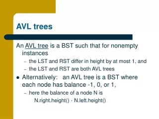
AVL trees An AVL tree is a BST such that for nonempty instances • the LST and RST differ in height by at most 1, and • the LST and RST are both AVL trees • Alternatively: an AVL tree is a BST where each node has balance -1, 0, or 1, • here the balance of a node N is N.right.height() - N.left.height()
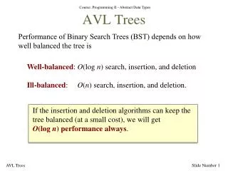
AVL tree height • An AVL tree of n has height O(log n) • note: ordinary BSTs can't make this guarantee • To see this, let N(h) be the smallest number of nodes in an AVL tree of height h. • then for h > 0, N(h) = 1 + N(h-1) + N(h-2) • a simple induction shows that N(h) > ah-1, where a = 1.5 • so for any AVL tree of height h>0, n > N(h) >= ah-1, • and then h <= 1 + logan, which is O(log n)
AVL tree operations • The search operation for ordinary BSTs may be used for AVL trees • Insertion for AVL trees is ordinary BST insertion followed by rebalancing • to restore the AVL property • Deletion is similar to insertion • we’ll say little about it
AVL tree insertion • After BST insertion but before rebalancing, the possible node balances are limited • they can only be -2, -1, 0, +1, or +2 • The balances -2 and +2 may only occur along the path to the newly inserted node. • It's enough to rebalance at the lowest node with one of these two balances • doing so will automatically fix all bad balances between that node and the root
AVL rebalancing as rotation • There are 5 possible binary trees of size n=3: LL LR RL RR • Only the middle one is an AVL tree • rebalancing simply makes the other 4 look like it • For larger n, subtrees go where they need to go to preserve the binary search property
AVL rotations • Recall that rotation is performed at a node • The LL, LR, RL, and RR cases are defined in terms of the balance at this node, and at the root of its higher subtree, as shown above • We’ll see shortly why these are the only possible cases • Note that there's a symmetry between right and left
AVL rotations in Weiss • Note that book's Figure 4.40 for LL differs from ours • Weiss is simply observing that one subtree moves as a unit • Note that an inorder traversal processes the nodes and subtrees in the same order after rotation as before • Note that LR rebalancing can be expressed as an RR rebalancing followed by an LL rebalancing
Claims about balance • Balances can only change if a height does • If balance changes at a node, then it must have changed everywhere below the node • since the height must change • also, all these lower nodes must have become more imbalanced.
Further claims about balance • At the point N of rotation, the balance must have changed from +1 to +2 or -1 to -2. • All nodes between N and the new node must have had a balance change to a legal value, • and hence from 0 to +1 or -1 • After each rotation, N has same height as before insertion.
Why 1 rotation gives an AVL tree • After insertion but before rotation, the nodes off the path to the new node are balanced • and rotation doesn’t change this • Rotation fixes the balance at N • Nodes below N were balanced before rotation (since N is the lowest bad node) • they do not become unbalanced by rotation • Those above this node remain balanced • since the appropriate subtree heights are the same after rotation as they were before insertion.
Splay trees • One possibly annoying feature of AVL trees is the need to check tree heights • So what if we just rotate without checking? • The intuition behind a splay tree: the most recently accessed node moves to the root • together with the LRU property , this is likely to make future accesses more efficient. • The motion is like AVL rotations, but new roots move two levels up even in single rotations
Splay tree rotations • There are 4 cases for rotation (LL, LR, RL, and RR), just as for AVL trees. • However the word zig is usually used instead of L, and zag instead of R. • The LR and RL cases are handled by the same double rotations as for AVL trees. • The LL and RR cases are handled by making the node the root, and letting the old parent and grandparent dangle to the right.
Applying splay tree rotations • These operations are applied repeatedly (moving the node 2 levels per operation) until the new node is at the root, or within one level of the root. • In the last case, the appropriate AVL single rotation then moves the node to the root. • Deletion of a node: • move node to root • rotate the max. node of LST the to the LST's root • insert the RST as the new RST of the LST
Efficiency of splay trees • Fact: Search, insertion, and deletion have amortized time complexity O(log n) • the proof is in Chapter 11 -- we won't cover it • cf. the amortized behavior of ArrayList.add • In the examples, note how spending time on one operation makes later operations easier
M-ary search trees • An m-ary search tree is an ordered tree where • Each nonleaf node has at most M children • A nonleaf with k children has k-1 keys. If the keys are indexed from 1 through k-1 and the subtrees from 0 through k-1, then • data items less than key 1 are in subtree 0 • data items between keys j and j+1 are in subtree j • data items greater than key k-1 are in subtree k-1
B-trees • A B-tree is an M-ary search tree where • all data items are stored in leaves • in a nonleaf, key i appears in subtree i • the root may have as few as 2 children, or be a leaf • nonleaves contain from M/2 to M children • leaves contain from L/2 to L data items • all leaves are at the same depth
B-tree pragmatics • We’re actually defining a B+ tree, by requiring that all data items be in leaves • The parameter L may be chosen based on hardware concerns (cf. Weiss, p. 149) • B-tree heights are logarithmic • For the same reason as for ordinary BSTs • In practice, they have very few levels • B-trees reduce the number of levels at the cost of extra work within a level • this makes sense only if external storage is used
Number of nodes in a B+-tree • For a B+-tree, the minimum number of nodes is • at level for m=L=100 for m=L=200 • 0 1 1 • 1 2 2 • 2 100 200 • 3 5,000 20,000 • 4 250,000 2,000,000
Number of keys in a B+-tree • If the level of the leaves is level k, then the minimum number of keys in a B+-tree is • k for m=L=100 for m=L=200 • 0 1 1 • 1 98 198 • 2 4,900 19,800 • 3 245,000 1,980,000 • 4 12,250,000 198,000,000
B-tree sizes and efficiency • Because of the rapid growth of size with height, B-tree heights are effectively O(1) • and thus so are search, insertion, and deletion • assuming that M and L are not too small • But in examples, we need small M and L • this makes over/underflow much more likely • if M = 3, the tree is often called a 2-3 tree • here nonleaves can have either 2 or 3 children • note that this applies to the root as well
B-tree operations • B-tree search is the natural generalization of BST search • B-tree insertion begins with the natural generalization of BST insertion, and then deals with any overflow • Note: that in B+-trees, all insertion is into leaves • B+-tree deletion removes from a leaf, and then deals with any underflow
Handling B+-tree overflow • Leaf overflow: • try passing a key to a sibling node • otherwise split and copy a key up • Nonleaf overflow: • try passing a key to a sibling node • otherwise split and pass a key up
Handling B+-tree underflow • Leaf underflow: • try getting a key or keys from a sibling node • otherwise merge and delete the separating key from the parent • Nonleaf underflow: • try getting a key or keys from a sibling node • otherwise merge and bring down the separating key from the parent
B+-tree algorithm details • Adding or deleting the first key of a leaf requires updating a nonleaf • Passing keys among siblings requires updating the separating key in their parent • Passing keys among siblings is tried first since several keys may be passed at once • also, splitting or merging may propagate
Correctness of splitting • Splitting a node during insertion gives a legal B+-tree, since: • If the node is a leaf • overflow gives a node with L+1 keys. • if they’re split evenly, each node gets at least L/2 • If the node is a nonleaf • replace “L” and “keys” with "M" and "children“ • any new root has 1 key and 2 children, so is legal
Correctness of underflow handling • In case of underflow during deletion: • If a leaf underflows (i.e., gets <= L/2 - 1 keys) • siblings with > L/2 + 1 keys can contribute keys • siblings with fewer keys can be merged with • If a nonroot nonleaf overflows • replace “L” and “keys” with "M" and "children“ • If the root underflows (i.e., gets 0 keys) • then 1 child remains -- make it the new root