Download
1 / 57
570 likes | 693 Vues
Statistics & Data Analysis. Course Number B01.1305 Course Section 31 Meeting Time Wednesday 6-8:50 pm. CLASS #5. Class #5 Outline. Understand random sampling and systematic bias Derive theoretical distribution of summary statistics Understand the Central Limit Theorem

E N D
Statistics & Data Analysis Course Number B01.1305 Course Section 31 Meeting Time Wednesday 6-8:50 pm CLASS #5
Class #5 Outline • Understand random sampling and systematic bias • Derive theoretical distribution of summary statistics • Understand the Central Limit Theorem • Use a normal probability plot to assess normality
Review of Last Class • Special Distributions • Counting problems • Binomial distribution problems • Normal distribution problems
CHAPTER 6 Random Sampling and Sampling Distributions
Chapter Goals • Explain why in many situations a sample is the only way learn something about a population • Explain the various methods of selecting a sample • Define and construct sampling distribution of sample means • Understand sources of bias or under-representation in data
A Scenario • Its 9:00 AM on Wednesday and your boss sent you and email asking how your firm’s customers would react to a new price discounting program • Your report is due tomorrow • It takes 10 minutes to interview a single customer in your database of almost 2,000 • What will you do???? • Draw a sample of the customers • How will you draw the sample? • Need a representative sample • Does your database hold a representative sample???
Background • Some previous chapters emphasized methods for describing data • Created frequency distributions, computed averages and measures of dispersion • Started to lay foundation for inference by studying probability • Counting, Binomial, and Normal Distributions • Probability distributions encompass all possible outcomes of an experiment and the probability associated with each outcome • So far, we’ve learned how to describe something that has already occurred or evaluate something that might occur
How are these similar… • QC department needs to check the tensile strength of steel wire • Five small pieces are selected every 5 hours • Tensile strength of each piece is determined • Marketing needs to determine the sales potential of a new drug named HappyPill. • 452 consumers were asked to try it for a week • Each consumer completed a questionnaire • Polling agency selections 2,000 voters at random and asked their approval rating of the President • In the study of insider trading, 25 CEOs were identified by the SEC and their trades were monitored for three years
Why Sample??? • Destructive nature of some tests • Physical Impossibility of checking all items • Cost of studying all items • Adequacy of sample results • Contacting whole population would be too time-consuming
Types of Samples • Cross-sectional: samples are taken from an underlying population at a particular time • Time-series: samples are taken over time from a random process • Enumerative Studies: sampling from a well-defined population • Analytic Studies: look at the results of a random process to predict future behavior
Why Sample??? • We often need to know something about a large population. • What is the average income of all Stern students? • It’s often too expensive and time-consuming to examine the entire population • Solution: Choose a small random sample and use the methods of statistical inference to draw conclusions about the population • Sampling lets us dramatically cut the costs of gathering information, but requires care. We need to ensure that the sample is representative of the population of interest • But how can any small sample be completely representative?
Why Sample (cont.) • IT IS IMPORTANT TO REALIZE THAT SOME INFORMATION IS LOST IF WE ONLY EXAMINE A SAMPLE OF THE ENTIRE POPULATION • Why not just use the sample mean in place of μ? • For example, suppose that the average income of 100 randomly selected Stern students was = 62,154 • Can we conclude that the average income of ALL Stern students (μ) is 62,154? • Can we conclude that μ > 60,000? • Fortunately, we can use probability theory to understand how the process of taking a random sample will blur the information in a population • But first, we need to understand why and how the information is blurred
Sampling Variability • Although the average income of all Stern Langone students is a fixed number, the average of a sample of 100 students depends on precisely which sample is taken. In other words, the sample mean is subject to “sampling variability” • The problem is that by reporting sample mean alone, we don’t take account of the variability caused by the sampling procedure. If we had polled different students, we might have gotten a different average income • It would be a serious mistake to ignore this sampling variability, and simply assume that the mean income of all students is the same as the average of the 100 incomes given in the sample
Populations and Samples • You are considering opening an Atomic Wings in Bethlehem, PA • POPULATION: All residents • SAMPLE: • Every 35th person at the mall • Every 2,000th person in the phone book • Every person who leaves Burger King • Don’t forget to include the college students!!!
Choosing a Representative Sample • REPRESENTATIVE: Each characteristic occurs in the same percentage of the time in the sample as in the population • BIAS: Not representative • Bias will exist if there is a systematic tendency to over/under represent some part of the population • By deliberately not sampling based on any specific characteristic, a randomly selected sample will typically be free from bias • Randomly selecting subjects lets you make probability statements about the results
Examples of Bias • Selection Bias: • A telephone survey of households conducted entirely between 9 a.m. to 5 p.m. • Using a customer complaint database to query on the new discount program • Nonresponse Bias: Sample member refuses to participate • Every market research program • Operational Definitions: Guiding a response • Do you agree that taxes are too high in New York
Simple Random Sampling • Process where each possible sample of a given size has the same probability of being selected • Example: IBM reported sales of $64.792 Billion and a net loss of $2.827 Billion for 1991. • The number of individual transactions was enormous • The auditors used statistics because to choose a representative sample of transactions to check in detail
Choosing a Random Sample • Number every member in the population 1…N • Use a random process to select the sample • R, flipping a coin, random number table…whatever is appropriate • In this class we will use the computer
Sampling Statistics and Distributions • Once a sample is drawn, we summarize it with sample statistics • The value of any summary statistic will vary from sample to sample (a big problem…no?) • A sample statistic is itself a random variable • Hence, it has a theoretical probability distribution called the sampling distribution • We can find the mean and standard deviation of many random samples
Example • Suppose the long-run average of the number of Medicare claims submitted per week to a regional office is 62,000, and the standard deviation is 7,000. • If we assume that the weekly claims submissions during a 4-week period constitute a random sample of size 4, what are the expected value and standard error of the average weekly number of claims over a 4-week period? • NOTE: Standard error denotes the theoretically derived standard deviation of the sampling distribution of a statistic.
Standard Error • Standard Deviation of the statistic • Is interpreted just as you would any standard deviation • Indicates approximately how far the observed value of the statistic is from its mean • Literally: it indicated the standard deviation you would find if you took a very large number of samples, found the sample average for each one, and worked with these sample averages as a data set
Example • Suppose n=200 randomly selected shoppers interviewed in a mall say they plan to spend on an average of $19.42 today with a standard deviation of $8.63 • This tells you what shoppers typically plan to spend, and that a typical, individual shopper plans to spend about $8.63 more or less than this amount • So far, this is no more that a description of the individuals interviewed • We can say something about the unknown population mean, which is the mean amount that all shoppers in the mall today plan to spend, including those not interviewed. • What is the standard error of the mean? • This tells us the variability when we use the sample average of $19.42, as an estimate of the unknown population mean
Sampling Distributions for Means and Sums • If a population distribution is Normal, then the sampling distribution of sample means is also Normal • Example: A timber company is planning to harvest 400 trees from a very large stand. • Yield is determined by its diameter • Distribution of diameters is normal with mean 44 inches and standard deviation of 4 inches • Find the probability that the average diameter of the harvest trees is between 43.5 and 44.5 inches.
Example • Its OK if each beer isn’t exactly 12 oz so long as the average volume isn’t too low or too high. • In your production facility, you know that the volume of each beer follows a Normal distribution, has a standard deviation of 0.5 ounces, representing variability about their mean of 12.01 oz. • Any case (24 beers) that has an average weight per beer less than 11.75 ounces will be rejected. • What fraction of cases will be rejected this way? • First find the mean and standard deviation of the average of n=24 beers
Central Limit Theorem • For any population, the sampling distribution of the sample mean is approximately normal if the sample size is sufficiently large
Simulation Example • Use R to draw 1000 samples each, with sample sizes 4, 10, 30, and 60 from a highly right-skewed distribution having mean and standard deviation both equal to 1. • Display a histogram of the sample means data=numeric(0) for (i in 1:1000) data[i] = mean( rexp(4) ) hist(data) • What type of process might follow this distribution???
Example of Use • An agency of the Commerce Department in a certain state wishes to check the accuracy of weights in supermarkets • They decide to weigh 9 packages of ground meat labeled as 1 pound packages • They will investigate any supermarket where the average weight of the packages is less than 15.5 oz • Assuming that the standard deviation of package weights is 0.6 oz, what is the probability they will investigate an honest market?
Normal Probability Plot • Plots actual versus expected values, assuming a normal distribution • Nearly normal data will plot as a near straight line • Right-skewed data plot as a curve, with the slope getting steeper as one moves to the right • Left-skewed data plot as a curve, with the slope getting flatter as one moves to the right • Symmetric but outlier-prone data plot as an S-shape, with the slope steepest at both sides
R Examples • data = rnorm(1000) ## do not worry about the r*** commands hist(data) qqnorm(data) qqline(data) • data = rexp(1000) hist(data) qqnorm(data) qqline(data) • data = 1-rlnorm(1000)+30 hist(data) qqnorm(data) qqline(data) • data = rnorm(1000); data[1]=5; data[2]=7; hist(data) qqnorm(data) qqline(data)
Point and Interval Estimation Chapter 7
Review • Basic problem of statistical theory is how to infer a population or process value given only sample data • Any sample statistic will vary from sample to sample • Any sample statistic will differ from the true, population value • Must consider random error in sample statistic estimation
Chapter Goals • Summarize sample data • Choosing an estimator • Unbiased estimator • Constructing confidence intervals for means with known standard deviation • Constructing confidence intervals for proportions • Determining how large a sample is needed • Constructing confidence intervals when standard deviation is not known • Understanding key underlying assumptions underlying confidence interval methods
Reminder: Statistical Inference • Problem of Inferential Statistics: • Make inferences about one or more population parameters based on observable sample data • Forms of Inference: • Point estimation: single best guess regarding a population parameter • Interval estimation: Specifies a reasonable range for the value of the parameter • Hypothesis testing: Isolating a particular possible value for the parameter and testing if this value is plausible given the available data
Point Estimators • Computing a single statistic from the sample data to estimate a population parameter • Choosing a point estimator: • What is the shape of the distribution? • Do you suspect outliers exist? • Plausible choices: • Mean • Median • Mode • Trimmed Mean
Example • I used R to draw 1,000 samples, each of size 30, from a normally distributed population having mean 50 and standard deviation 10. • For each sample the mean and median are computed. data.mean = numeric(0) data.median = numeric(0) for(i in 1:1000) { data = rnorm(30, mean=50, sd=10) data.mean[i] = mean(data) data.median[i] = median(data) } • Do these statistics appear unbiased? • Which is more efficient?
Confidence Interval • An interval with random endpoints which contains the parameter of interest (in this case, μ) with a pre-specified probability, denoted by 1 - α. • The confidence interval automatically provides a margin of error to account for the sampling variability of the sample statistic. • Example: A machine is supposed to fill “12 ounce” bottles of Guinness. To see if the machine is working properly, we randomly select 100 bottles recently filled by the machine, and find that the average amount of Guinness is 11.95 ounces. Can we conclude that the machine is not working properly?
No! By simply reporting the sample mean, we are neglecting the fact that the amount of beer varies from bottle to bottle and that the value of the sample mean depends on the luck of the draw • It is possible that a value as low as 11.75 is within the range of natural variability for the sample mean, even if the average amount for all bottles is in fact μ = 12 ounces. • Suppose we know from past experience that the amounts of beer in bottles filled by the machine have a standard deviation of σ = 0.05 ounces. • Since n = 100, we can assume (using the Central Limit Theorem) that the sample mean is normally distributed with mean μ (unknown) and standard error 0.005 • What does the Empirical Rule tell us about the average volume of the sample mean?
Confidence Intervals • “Statistics is never having to say you're certain”. • (Tee shirt, American Statistical Association). • Any sample statistic will vary from sample to sample • Point estimates are almost inevitably in error to some degree • Thus, we need to specify a probable range or interval estimate for the parameter
Example • An airline needs an estimate of the average number of passengers on a newly scheduled flight • Its experience is that data for the first month of flights are unreliable, but thereafter the passenger load settles down • The mean passenger load is calculated for the first 20 weekdays of the second month after initiation of this particular flight • If the sample mean is 112 and the population standard deviation is assumed to be 25, find a 90% confidence interval for the true, long-run average number of passengers on this flight
Interpretation • The significance level of the confidence interval refers to the process of constructing confidence intervals • Each particular confidence interval either does or does not include the true value of the parameter being estimated • We can’t say that this particular estimate is correct to within the error • So, we say that we have a XX% confidence that the population parameter is contained in the interval • Or…the interval is the result of a process that in the long run has a XX% probability of being correct
Imagine Many Samples Other intervals you might have computed Missed! Missed! The interval you computed 22 23 24 The population mean = 23.29
Getting Realistic • The population standard deviation is rarely known • Usually both the mean and standard deviation must be estimated from the sample • Estimate with s • However…with this added source of random errors, we need to handle this problem using the t-distribution (later on)
Confidence Intervals for Proportions • We can also construct confidence intervals for proportions of successes • Recall that the expected value and standard error for the number of successes in a sample are: • How can we construct a confidence interval for a proportion?
Example • Suppose that in a sample of 2,200 households with one or more television sets, 471 watch a particular network’s show at a given time. • Find a 95% confidence interval for the population proportion of households watching this show.