Download

1 / 36
360 likes | 2.44k Vues
HWRF Initialization -GSI customization. Mingjing Tong NOAA/NCEP/EMC 2014 Hurricane WRF Tutorial , January 14, NCWCP. Outline. Data assimilation upgrades for FY13 HWRF One-way hybrid ensemble-variational data assimilation system for HWRF

E N D
HWRF Initialization -GSI customization Mingjing Tong NOAA/NCEP/EMC 2014 Hurricane WRF Tutorial, January 14, NCWCP
Outline • Data assimilation upgrades for FY13 HWRF • One-way hybrid ensemble-variational data assimilation system for HWRF • Assimilation of NOAA-P3 Tail Doppler Radar (TDR) observation • GSI customization • Setup hybrid analysis • First guess (FGAT) • Observations • GSI namelist • GSI fix files • GSI standard output • Observation fitting statistics
HWRF domains GSI analysis domain 43 vertical levels with 50 hPa model top Model forecast domains outer domain: 216x432 – 80°x80° ; 0.18° middle nest: 88x170 – 11°x10°; 0.06° inner nest: 180x324 – 7.2°x6.5°; 0.02° HWRF vortex initialization domain 3x domain: 748x1504 – 30°x30° GSI analysis domain: outer domain ghost d03: 529x988 - 20°x20°; 0.02° After GSI analysis, model fields in ghost d03 are interpolated to inner nest, middle nest and outer domain. The area between ghost d03 and middle nest is a blending zone, where ghost domain analysis gradually merged to outer domain analysis. HWRF domains (Fig 4.1 of HWRF USERS’ GUIDE)
Assimilation System • First guess • Outer domain: GDAS forecast after relocation • ghost d03: GDAS forecast (TC environment) + modified GDAS/HWRF vortex • Hybrid data assimilation configuration • 80 ensemble member at T254L64 • outer domain β1-1=0.25 – ¼ static and ¾ ensemble covariance horizontal localization: 1546km gradually increase to 2320 km from around 276 hPa (27th model level) and above vertcial localization: 1.2 in natural log of pressure • ghost d03 β1-1=0.2 – 1/5 static and 4/5 ensemble covariance horizontal localization: 387 km E-folding vertical localization: 10 vertical model levels for weak storms and 20 vertical model levels for strong storms (equal or greater than category 1)
Assimilation System • GSI analysis variables • Analysis variables used for HWRF include streamfunction (ψ), velocity potential (χ), temperature (T), surface pressure (Ps), normalized relative humidity, satellite bias correction coefficients • ozone and cloud variables are not analyzed for FY13 HWRF • Model variables updated • u, v, t, q, pd, pint
Assimilation System • Observational data • Conventional observations assimilated in the HWRF outer and ghost domains include: • Radiosondes • Dropsondes • Aircraft reports (AIREP/PIREP, RECCO , MDCRS-ACARS, TAMDAR , AMDAR) • Surface ship and buoy observations • Surface observations over land • Pibal winds • Wind profilers • VAD wind • WindSat scatterometer winds • GPS-derived integrated precipitable water • NOAA P3 Tail Doppler Radar radial wind (TDR) data assimilated in ghost domain
Assimilation of NOAA-P3 Tail Doppler Radar Data 200 km P-3 regular Jorgensen et al., 1983, J. Climate Appl. Meteor, 22, 744-757 400 km P-3 weak storm P-3 weak storm
Assimilation of NOAA-P3 Tail Doppler Radar (TDR) Radial Velocity Data • TDR data are assimilate in ghost domain after vortex initialization • Data with innovation (o-f) greater than 20 m/s are rejected • Observation error is 5 m/s and gradually increases to 10 m/s as o-f is greater than 10 m/s • Reject small data dump at the ends of assimilation window • Data thinned to 9 km horizontal resolution • Assimilation time window – analysis time ±3 hours • To deal with the distribution of the inner core observations in hours of time window within 3D data assimilation framework, FGAT (First Guess at Appropriate Time) is used assimilation window -6 hr -3 hr +3 hr 0 hr * FGAT - compares observations with the background at the observation time; In traditional 3DVAR scheme, observation is assumed to be valid at the analysis time and is used to compute the innovation
Impact of TDR data assimilation First guess at 850 hPa Analysis at 850 hPa Analysis at 850 hPa First guess vortex is much bigger than observed vortex HWRF analysis is consistent with HRD wind analysis
with TDR TDR innovation without TDR
Setup DA configuration in /glade/scratch/$USER/HWRF_v3.5a/sorc/hwrf-utilities/wrapper_scripts/global_vars.ksh BKG_MODE=GDAS # Define first guess If BKG_MODE=GFS means using GFS analysis and GSI will be turned off RUN_GSI=T # T run GSI data assimilation RUN_GSI_WRFINPUT=T # T run GSI DA for outer domain RUN_GSI_WRFGHOST=F # T run GSI DA for ghost domain INNER_CORE_DA=1 # 0=no inner core DA; 1=TDR only; 2=HDOB only; 3=TDR and HDOB If INNER_CORE_DA > 0 and inner core data are found, RUN_GSI_WRFGHOST will be ignored and assumed T by other scripts, even if RUN_GSI_WRFGHOST=F in global_vars.ksh If RUN_GSI_WRFGHOST=T, always turn on GSI for ghost domain, no matter whether there is inner core data or not FGAT=“-3,0,3” # FGAT window times relative to analysis time GSI_ENS_REG=T # Option to run hybrid DA F = 3DVAR DA GSI_ENS_REG_OPT=1 # Using global EnKF-3DVAR hybrid ensemble for HWRF hybrid DA GSI_ENS_REG_SIZE=80 # Number of ensemble members Data Assimilation Configuration
Setup hybrid DA in GSI script function main { … if [[ "$GSI_ENS_REG" =~ ^[Tt] ]] ; then # using global ensemble cp_ens fi … } • Link ensemble forecast files function cp_ens { typeset -Z3 n=1 typeset d typeset jdn typeset p typeset f typeset x=0 jdn=$(jdn ${START_TIME} ) (( jdn -= (${FCST_INTERVAL} / 24.0) )) p=$(gtime -s $jdn) d=${GEFS_ENS_FCST_DIR}/${p:0:10} if [[ "$GSI_ENS_REG" =~ ^[T|t] \ && "$GSI_ENS_REG_OPT" -eq 1 ]] ; then while [[ $n -le ${GSI_ENS_REG_SIZE} ]]; do f=${d}/sfg_${p:0:10}_fhr06s_mem${n} if [ -f $f ] ; then ${LS} $f >> filelist # * (( ++x )) fi (( ++n )) done if [ $x -eq 0 ]; then error "No ensemble member files found." fi fi } * GSI read in global ensemble by first read in the file ‘filelist’ and then the files listed in filelist
Setup hybrid DA in GSI script 2. GSI namelist &HYBRID_ENSEMBLE l_hyb_ens=HYBENS_REGIONALVALUE, ! If true, then turn on hybrid ensemble option n_ens=80, ! Number of ensemble members uv_hyb_ens=.true., ! True for regional model beta1_inv=0.2, ! Weight given to static background error covariance (0 <= beta1_inv<=1) s_ens_h=HYBENS_HOR_SCALE_REGIONALVALUE, !Horizontal localization length scale (km) s_ens_v=HYBENS_VER_SCALE_REGIONALVALUE, !Vertical localization length scale (lnP or grid units) ! If in lnP, s_ens_v need to be a negative number readin_localization=.false.; ! Flag to read in external localization information file !(hybens_locinfo) generate_ens=.false., regional_ensemble_option=REGIONAL_ENSEMBLE_OPTIONVALUE, ! 1 use global ensemble internally interpolated to ensemble grid. ! 2 ensembles are WRF NMM format (HWRF) grid_ratio_ens=1, ! For regional runs, ratio of ensemble grid to analysis grid resolution pseudo_hybens=.false., merge_two_grid_ensperts=.false., pwgtflg=.false., betaflg=.false., aniso_a_en=.false., nlon_ens=NLON_ENS_REGIONALVALUE, nlat_ens=NLAT_ENS_REGIONALVALUE, jcap_ens=0, jcap_ens_test=0, /
First Guess (FGAT) # Copy the WRF input and output file(s) for domain wrfghost function cp_wrfghost{ … if [ "${BKG_MODE}" = "GDAS" ]; then if [ $(check_inner_da) = "true" ] ; then for i in {$FGAT} ; do j=$(otime -o $i ${START_TIME} ) (( k = FCST_INTERVAL + i )) src=${DOMAIN_DATA}/relocateprd/${j:0:10} if [ $i -eq 0 ]; then dst=wrf_inout#Copy first guess valid at analysis time else dst=wrf_inou$k#Copy first guess at other time levels for FGAT fi #i.e. as wrfinou3, wrfinou9 # $k is forecast hour dfile=wrfghost_d02 copy $src/${dfile} $dst done else … }
Observations – control data usage • Presence or lack of input data cp $datobs/${prefixa}.prepbufr ./prepbufr conventional data cp $datobs/${prefixo}.tldplr.${suffix} ./tldplrbufr TDR data cp $datobs/${prefixa}.goesfv.${suffix} ./gsnd1bufr cp $datobs/${prefixa}.1bamua.${suffix} ./amsuabufr cp $datobs/${prefixa}.1bamub.${suffix} ./amsubbufr cp $datobs/${prefixa}.1bhrs3.${suffix} ./hirs3bufr satellite data cp $datobs/${prefixa}.1bhrs4.${suffix} ./hirs4bufr cp $datobs/${prefixa}.1bmhs.${suffix} ./mhsbufr cp $datobs/${prefixa}.airsev.${suffix} ./airsbufr
Observations – control data usage • GSI namelist &OBS_INPUT dmesh(1)=120.0,dmesh(2)=60.0,dmesh(3)=60.0,dmesh(4)=60.0,dmesh(5)=120, dmesh(7)=9.0, time_window_max=$twind, dfile(01)='prepbufr', dtype(01)='ps', dplat(01)=' ', dsis(01)='ps', dval(01)=0.0, dthin(01)=0, dsfcalc(01)=0, dfile(02)='prepbufr' dtype(02)='t', dplat(02)=' ', dsis(02)='t', dval(02)=0.0, dthin(02)=0, dsfcalc(02)=0, dfile(03)='prepbufr', dtype(03)='q', dplat(03)=' ', dsis(03)='q', dval(03)=0.0, dthin(03)=0, dsfcalc(03)=0, dfile(04)='prepbufr', dtype(04)='pw', dplat(04)=' ', dsis(04)='pw', dval(04)=0.0, dthin(04)=0, dsfcalc(04)=0, dfile(05)='prepbufr', dtype(05)='uv', dplat(05)=' ', dsis(05)='uv', dval(05)=0.0, dthin(05)=0, dsfcalc(05)=0, dfile(06)='satwndbufr',dtype(06)='uv', dplat(06)=' ', dsis(06)='uv', dval(06)=0.0, dthin(06)=0, dsfcalc(06)=0, dfile(07)='prepbufr', dtype(07)='spd', dplat(07)=' ', dsis(07)='spd', dval(07)=0.0, dthin(07)=0, dsfcalc(07)=0, dfile(08)='prepbufr', dtype(08)='dw', dplat(08)=' ', dsis(08)='dw', dval(08)=0.0, dthin(08)=0, dsfcalc(08)=0, dfile(09)='radarbufr', dtype(09)='rw', dplat(09)=' ', dsis(09)='rw', dval(09)=0.0, dthin(09)=0, dsfcalc(09)=0, dfile(10)='prepbufr', dtype(10)='sst', dplat(10)=' ', dsis(10)='sst', dval(10)=0.0, dthin(10)=0, dsfcalc(10)=0, dfile(11)='tcvitl' dtype(11)='tcp', dplat(11)=' ', dsis(11)='tcp', dval(11)=0.0, dthin(11)=0, dsfcalc(11)=0, ……. dfile(23)='hirs3bufr', dtype(23)='hirs3', dplat(23)='n17', dsis(23)='hirs3_n17', dval(23)=0.0, dthin(23)=1, dsfcalc(23)=0, dfile(24)='hirs4bufr', dtype(24)='hirs4', dplat(24)='metop-a', dsis(24)='hirs4_metop-a', dval(24)=0.0, dthin(24)=1, dsfcalc(24)=1, dfile(25)='gimgrbufr', dtype(25)='goes_img', dplat(25)='g11', dsis(25)='imgr_g11', dval(25)=0.0, dthin(25)=1, dsfcalc(25)=0, …… dfile(67)='amsuabufr', dtype(67)='amsua', dplat(67)='metop-b', dsis(67)='amsua_metop-b', dval(67)=0.0, dthin(67)=2, dsfcalc(67)=0, dfile(68)='mhsbufr', dtype(68)='mhs', dplat(68)='metop-b', dsis(68)='mhs_metop-b', dval(68)=0.0, dthin(68)=3, dsfcalc(68)=0, dfile(69)='iasibufr', dtype(69)='iasi', dplat(69)='metop-b', dsis(69)='iasi616_metop-b', dval(69)=0.0, dthin(69)=1, dsfcalc(69)=0, …… dfile(78)='gsnd1bufr', dtype(78)='sndrd2', dplat(78)='g15', dsis(78)='sndrD2_g15', dval(78)=0.0, dthin(78)=5, dsfcalc(78)=0, dfile(79)='gsnd1bufr', dtype(79)='sndrd3', dplat(79)='g15', dsis(79)='sndrD3_g15', dval(79)=0.0, dthin(79)=5, dsfcalc(79)=0, dfile(80)='gsnd1bufr', dtype(80)='sndrd4', dplat(80)='g15', dsis(80)='sndrD4_g15', dval(80)=0.0, dthin(80)=5, dsfcalc(80)=0, horizontal resolution (km) of TDR data thinning grid radar data including TDR
Observations – control data usage 3. GSI info/fix files • convinfo (for conventional data) !otype type sub iusetwindownumgrpngroupnmiter gross ermaxerminvar_bvar_pgithinrmeshpmeshnpred ps 111 0 -1 1.5 0 0 0 5.0 3.0 1.0 10.0 0.000 0 0. 0. 0 ps 120 0 1 1.5 0 0 0 5.0 3.0 1.0 10.0 0.000 0 0. 0. 0 ps 132 0 -1 1.5 0 0 0 5.0 3.0 1.0 10.0 0.000 0 0. 0. 0 … rw 999 0 10.5 0 0 0 5.0 10.0 2.0 10.0 0.000 0 0. 0. 0 … • satinfo (for satellite data) sensor/instr/sat chaniuse error ermaxvar_bvar_pg amsua_n15 1 1 3.000 4.500 10.00 0.000 amsua_n15 2 1 2.000 4.500 10.00 0.000 amsua_n15 3 1 2.000 4.500 10.00 0.000 amsua_n15 4 1 0.600 2.500 10.00 0.000 amsua_n15 5 1 0.300 2.000 10.00 0.000 amsua_n15 6 1 0.230 2.000 10.00 0.000 using radar data
Conventional Data • Dropsonde wind observations within max(111km, 3xRMW) were flagged (not used) • Surface pressure data within the vortex area are flagged • Data remove program – hwrf_data_remv (not used in FY13 HWRF) Input RRADC – radius from TC center Function Remove all conventional data within RRADC km from TC center • Data flag program – hwrf_data_flag Input RRADC - radius from TC center for dropsonded wind RBLDC - radius from TC center for surface pressure data Function Change the data usage flag from use to not use
GSI fix files • background error covariance cp$GSI_FIXED_DIR/nam_glb_berror.f77.gcv ./berror_stats • observation error table cp$GSI_FIXED_DIR/prepobs_errtable.hwrf ./errtable • Radiance coefficient used by CRTM cp$GSI_CRTM_FIXED_DIR/EmisCoeff.bin ./EmisCoeff.bin cp$GSI_CRTM_FIXED_DIR/AerosolCoeff.bin ./AerosolCoeff.bin cp$GSI_CRTM_FIXED_DIR/CloudCoeff.bin ./CloudCoeff.bin
GSI fix files • Observation data control file cp$GSI_FIXED_DIR/nam_regional_convinfo.txt ./convinfo cp$GSI_FIXED_DIR/nam_regional_satinfo.txt ./satinfo cp $GSI_FIXED_DIR/nam_global_pcpinfo.txt ./pcpinfo cp $GSI_FIXED_DIR/nam_global_ozinfo.txt ./ozinfo satinfo, pcpinfo and ozinfo are not used, because satellite radiance data, ozone data and precipitation rate observations are not assimilated into FY13 HWRF • Satellite bias correction coefficients cp$GSI_FIXED_DIR/gdas.t${CYCLE}z.satang ./satbias_angle cp$GFS_OBS_DIR/gdas.t${CYCLE}z.abias ./satbias_in
GSI namelist &SETUP miter=2,niter(1)=50,niter(2)=50, * two outer loop with 50 iterations each write_diag(1)=.true.,write_diag(2)=.false.,write_diag(3)=.true., * output innovation diagnostic information gencode=78,qoption=2, * use normalized relative humidity as analysis variable ndat=16, * number of data listed in &OBS_INPUT oneobtest=.false.,retrieval=.false., nhr_assimilation=6,l_foto=.false., use_pbl=.true.,
GSI namelist &GRIDOPTS JCAP=$JCAP,JCAP_B=$JCAP_B,NLAT=$NLAT,NLON=$LONA,nsig=$LEVS, * analysis domain dimensions. It’s okay if wrong values are given to NLAT, NLON and nsig. For HWRF, domain dimensions are read in from input background data hybrid=.true.,wrf_nmm_regional=.true.,wrf_mass_regional=.false., * if run GSI for HWRF, need to be set to ‘true’. ‘hybrid’ means hybrid vertical coordinates, not hybrid analysis &BKGERR as=1.0,1.0,0.5 ,0.7,0.7,0.5,1.0,1.0, vs=1.0 hzscl=0.373,0.746,1.50, * static background error variance and correlation length scale parameter bw=0.,fstat=.true., &ANBKGERR anisotropic=.false., * anisotropic static background error covariance is not used for FY13 HWRF
GSI namelist &JCOPTS &STRONGOPTS jcstrong=.false., * TLNMC constraint (Kleist et. al. 2009)is not used for HWRF &OBSQC dfact=0.75,dfact1=3.0,noiqc=.false. &OBS_INPUT dmesh(1)=120.0,dmesh(2)=60.0,dmesh(3)=60.0,dmesh(4)=60.0,dmesh(5)=120,dmesh(9)=9,time_window_max=1.5, * dmesh – data thinning mesh size (km) * time_window_max– observation time window
“GSI Diagnostic” by Ming Hu, 2010 GSI tutorial Standard Output Details in User’s Guide Section 4.1 Highlight several important points
“GSI Diagnostic” by Ming Hu, 2010 GSI tutorial Check Background Input ZNW, RDX, RDY, MAPFAC_M, XLAT, XLONG, MUB, MU, PHB • 0: rmse_var=T • 0: ordering=XYZ • 0: WrfType,WRF_REAL= 104 104 • 0: ndim1= 3 • 0: staggering= N/A • 0: start_index= 1 1 1 -7269735 • 0: end_index= 69 64 45 -7269735 • 0: k,max,min,mid T= 1 309.9411316 264.5114136 289.7205811 • 0: k,max,min,mid T= 2 310.6200562 269.5698547 295.0413208 • 0: k,max,min,mid T= 3 311.5386047 272.4312744 296.7247009 • 0: k,max,min,mid T= 43 486.2092896 436.1306763 461.4866943 • 0: k,max,min,mid T= 44 498.1362000 456.4700012 478.7089233 • 0: k,max,min,mid T= 45 510.0127563 472.5627441 494.7407227 Variable name in netcdf file K Maximum Minimum Central grid QVAPOR, U, V, LANDMASK, XICE, SST,IVGTYP, ISLTYP, VEGFRA, SNOW, U10, V10, SMOIS, TSLB, TSK
“GSI Diagnostic” by Ming Hu, 2010 GSI tutorial Check Fix Files Input convinfo 0:READ_CONVINFO: ps120 0 1 3.0 0 0 0 4.0 3.0 1.0 4.0 0:READ_CONVINFO: ps132 0 -1 3.0 0 0 0 4.0 3.0 1.0 4.0 0:READ_CONVINFO: t 120 0 1 3.0 0 0 0 8.0 5.6 1.3 8.0 0:READ_CONVINFO: t 180 0 1 3.0 0 0 0 7.0 5.6 1.3 7.0 0:READ_CONVINFO: uv 220 0 1 3.0 0 0 0 8.0 6.0 1.4 8.0 0:READ_CONVINFO: uv 280 0 1 3.0 0 0 0 6.0 6.1 1.4 6.0 0:READ_CONVINFO: spd 283 0 1 3.0 0 0 0 8.0 6.1 1.4 8.0 CRTM coefficients 0: Read_SpcCoeff_Binary(INFORMATION) : FILE: ./hirs3_n16.SpcCoeff.bin; 0: SpcCoeff RELEASE.VERSION: 7.01 N_CHANNELS=19 0: Read_TauCoeff_Binary(INFORMATION) : FILE: ./hirs3_n16.TauCoeff.bin; 0: TauCoeff RELEASE.VERSION: 5.04 N_ORDERS=10 N_PREDICTORS= 6 N_ABSORBERS= 3 N_CHANNELS= 19 N_SENSORS= 1 0: Read_CloudCoeff_Binary(INFORMATION) : FILE: ./CloudCoeff.bin; 0: CloudCoeff RELEASE.VERSION: 2.02 N_FREQUENCIES(MW)= 31 N_FREQUENCIES(IR)= 701 N_RADII(MW)= 6 N_RADII(IR)= 6 N_TEMPERATURES= 5 N_DENSITIES= 3 N_LEGENDRE_TERMS=38 N_PHASE_ELEMENTS= 6
“GSI Diagnostic” by Ming Hu, 2010 GSI tutorial Check Observations Input 0: READ_OBS: read 1 ps ps using ntasks= 1 0 2 1 0: READ_OBS: read 2 t t using ntasks= 1 0 3 1 0: READ_OBS: read 3 q q using ntasks= 1 0 0 1 0: READ_OBS: read 4 uv uv using ntasks= 1 0 1 1 0: READ_OBS: read 5 spd spd using ntasks= 1 0 2 1 0: READ_OBS: read 7 dw dw using ntasks= 1 0 3 1 0: READ_OBS: read 8 sst sst using ntasks= 1 0 0 1 READ_PREPBUFR: messages/reports = 681 / 71658 ntread = 1 READ_PREPBUFR: file=prepbufr type=t sis=t nread= 11452 ithin= 0 rmesh=120.000 isfcalc= 0 ndata= 11280 ntask= 1 READ_PREPBUFR: messages/reports = 681 / 71658 ntread = 1 READ_PREPBUFR: file=prepbufr type=q sis=q nread= 11379 ithin= 0 rmesh=120.000 isfcalc= 0 ndata= 10186 ntask= 1 Observation distribution in an analysis using 4 processors 3:OBS_PARA: ps 291 508 1140 1561 3:OBS_PARA: t 484 887 1730 2729 3:OBS_PARA: q 464 868 1642 2568 3:OBS_PARA: uv 1146 2067 2766 5162 3:OBS_PARA: sst 0 0 47 0 3:OBS_PARA: pw 13 18 44 17 3:OBS_PARA: hirs3 n16 21 21 0 0 3:OBS_PARA: amsua n15 179 189 149 224
“GSI Diagnostic” by Ming Hu, 2010 GSI tutorial Check outer loop and inner iteration Inner iteration 1st outer loop 0:grepcost J,Jb,Jo,Jc,Jl = 1 01.6048921E+04 0.0E+0 1.60489216E+04 0.0E+0 0.0E+0 0:grepgrad grad,reduction= 1 0 4.622906854790679176E+02 1.000000000000000000E+00 0:pcgsoi: cost,grad,step = 1 0 1.60489216E+04 4.6229068547E+02 1.4816403979E-02 0:pcgsoi: gnorm(1:2),b= 1.24089076555E+05 1.240890765553E+05 5.8063507409044E-01 0: stprat 0.518838814777991403E-01 0: stprat 0.246311812999037177E-15 0: Minimization iteration 1 0:grepcost J,Jb,Jo,Jc,Jl = 1 11.288246E+04 4.6915E+01 1.283555E+04 0.0E+0 0.0E+0 0:grepgrad grad,reduction= 1 1 3.522627947361617657E+02 7.619941430814570760E-01 0:pcgsoi: cost,grad,step = 1 1 1.288246824862E+04 3.522627947E+02 1.408558895E-02 0:pcgsoi: gnorm(1:2),b= 3.9226971306926E+04 3.9226971306926E+04 3.1611945544163E-01 0: stprat 0.364906062575707624 0: stprat 0.156431139151674278E-14224 2nd outer loop Inner iteration 0: Minimization iteration 0 0:grepcost J,Jb,Jo,Jc,Jl = 2 09.9610405E+03 8.5076644E+02 9.1102740E+03 0.0 0.0 0:grepgrad grad,reduction= 2 0 2.291813874420873560E+02 1.000000000000000000E+00 0:pcgsoi: cost,grad,step = 2 0 9.96104052193E+03 2.29181387442E+02 7.15279261E-03 0:pcgsoi: gnorm(1:2),b= 1.13035507282E+04 1.13035507282E+04 2.15206903713E-01 0: stprat 0.319264972580440953 0: stprat 0.577830902990640559E-14 0: Minimization iteration 1 0:grepcost J,Jb,Jo,Jc,Jl = 2 19.58534646E+03 8.7366356E+02 8.7116829E+03 0.0 0.0 0:grepgrad grad,reduction= 2 1 1.063181580364677217E+02 4.639039811351767240E-01 0:pcgsoi: cost,grad,step = 2 1 9.58534646763E+03 1.06318158036E+02 1.05074549E-02 0:pcgsoi: gnorm(1:2),b= 5.4234537548554E+03 5.4234537548554E+03 4.7980089488985E-01 0: stprat 0.410968433100896591 0: stprat 0.157538354385690312E-13
“GSI Diagnostic” by Ming Hu, 2010 GSI tutorial Check Analysis Result Output 0: ordering=XY 0: WrfType,WRF_REAL= 104 104 0: ndim1= 2 0: staggering= N/A 0: start_index= 1 1 1 -7269735 0: end_index1= 69 64 45 -7269735 0: k,max,min,mid T= 1 309.9584656 264.4796753 290.9471130 0: k,max,min,mid T= 2 310.6225281 269.6447144 296.2458191 0: k,max,min,mid T= 44 496.4794922 457.3758850 478.2719116 0: k,max,min,mid T= 45 509.2687378 475.0305481 494.7050171 0: rmse_var=T K Maximum Minimum Central grid QVAPOR, U, V, SMOIS, XICE, SST, TSK Variable name in netcdf file
“GSI Diagnostic” by Ming Hu, 2010 GSI tutorial Observation Fitting Statistic Details in User’s Guide Section 4.5 “GSI Diagnostic” by Ming Hu, 2010 GSI tutorial
“GSI Diagnostic” by Ming Hu, 2010 GSI tutorial Why need to check fitting statistic • Data Analysis: adjust background fields based on observation data so that analysis fields fit the observation better. • GSI has a series of text files to provide statistic information on how outer loop fields fit to the certain observation variable (fort.2*) • GSI also has a series of binary files to save diagnostic information for each observation (diag*)
“GSI Diagnostic” by Ming Hu, 2010 GSI tutorial Statistic fitting files File names are from fort.201 to fort.215 (or fit_*) Each file is for one observation variable
“GSI Diagnostic” by Ming Hu, 2010 GSI tutorial Statistic fitting files (Continue) Satellite radiance Radar radial wind GPS RO
“GSI Diagnostic” by Ming Hu, 2010 GSI tutorial Example: fit_t1.2010050700 (fort.203) current fit of temperature data, ranges in K ptop 1000.0 900.0 800.0 600.0 400.0 300.0 250.0 200.0 150.0 100.0 50.0 0.0 it obs type styppbot 1200.0 999.9 899.9 799.9 599.9 399.9 299.9 249.9 199.9 149.9 99.9 2000.0 ------------------------------------------------------------------------------------------------------------------------- o-g01t120 0000 count 44 180 214 381 405 200 93 147 247 334 396 3432 o-g 01 t 120 0000 bias 3.67 2.12 0.51 0.23 -0.33 -0.63 -0.66 -1.49 -0.45 -1.04 -1.21 -0.40 o-g 01 t 120 0000 rms 4.36 2.77 1.45 1.19 0.83 1.04 1.43 2.09 1.74 1.89 2.38 1.81 o-g 01 t 130 0000 count 0 0 0 0 0 0 3 12 2 0 0 18 o-g 01 t 130 0000 bias 0.00 0.00 0.00 0.00 0.00 0.00 -0.55 -0.50 2.33 0.00 0.00 -0.04 o-g 01 t 130 0000 rms 0.00 0.00 0.00 0.00 0.00 0.00 0.57 1.31 2.51 0.00 0.00 1.48 o-g 01 t 180 0000 count 714 79 0 0 0 0 0 0 0 0 0 793 o-g 01 t 180 0000 bias 2.65 -0.03 0.00 0.00 0.00 0.00 0.00 0.00 0.00 0.00 0.00 2.38 o-g 01 t 180 0000 rms 3.66 1.56 0.00 0.00 0.00 0.00 0.00 0.00 0.00 0.00 0.00 3.51 o-g 01 all count 758 259 214 381 405 200 96 159 249 334 396 4243 o-g 01 all bias 2.70 1.46 0.51 0.23 -0.33 -0.63 -0.65 -1.41 -0.42 -1.04 -1.21 0.12 o-g 01 all rms 3.70 2.47 1.45 1.19 0.83 1.04 1.41 2.04 1.74 1.89 2.38 2.23 O-B current fit of temperature data, ranges in K ptop 1000.0 900.0 800.0 600.0 400.0 300.0 250.0 200.0 150.0 100.0 50.0 0.0 it obs type styppbot 1200.0 999.9 899.9 799.9 599.9 399.9 299.9 249.9 199.9 149.9 99.9 2000.0 -------------------------------------------------------------------------------------------------------------------------- o-g03t120 0000 count 44 180 214 381 405 200 93 147 247 334 396 3432 o-g 03 t 120 0000 bias 2.38 1.36 0.13 0.13 -0.07 -0.10 -0.03 -0.50 0.03 -0.24 -0.27 0.02 o-g 03 t 120 0000 rms 2.75 1.94 1.06 0.90 0.59 0.61 1.02 1.23 1.37 1.19 1.90 1.34 o-g 03 t 130 0000 count 0 0 0 0 0 0 3 12 2 0 0 18 o-g 03 t 130 0000 bias 0.00 0.00 0.00 0.00 0.00 0.00 -0.06 -0.04 1.70 0.00 0.00 0.29 o-g 03 t 130 0000 rms 0.00 0.00 0.00 0.00 0.00 0.00 0.26 1.08 1.87 0.00 0.00 1.24 o-g 03 t 180 0000 count 714 79 0 0 0 0 0 0 0 0 0 793 o-g 03 t 180 0000 bias 0.84 -0.21 0.00 0.00 0.00 0.00 0.00 0.00 0.00 0.00 0.00 0.74 o-g 03 t 180 0000 rms 2.34 1.38 0.00 0.00 0.00 0.00 0.00 0.00 0.00 0.00 0.00 2.27 o-g 03 all count 758 259 214 381 405 200 96 159 249 334 396 4243 o-g 03 all bias 0.93 0.88 0.13 0.13 -0.07 -0.10 -0.03 -0.46 0.04 -0.24 -0.27 0.16 o-g 03 all rms 2.37 1.79 1.06 0.90 0.59 0.61 1.01 1.22 1.37 1.19 1.90 1.56 O-A Results from test case using 2 outer loops with 10 inner iterations in each outer loop
“GSI Diagnostic” by Ming Hu, 2010 GSI tutorial Observation departure for each obs diag_amsua_metop-a_anl.2010050700 diag_amsub_n16_anl.2010050700 diag_amsua_metop-a_ges.2010050700 diag_amsub_n16_ges.2010050700 diag_amsub_n17_anl.2010050700 diag_conv_anl.2010050700 Diag_amsub_n17_ges.2010050700 diag_conv_ges.2010050700 • Diagnostic files: • To get these files, has to turn write_diag on: write_diag(1)=.true.,write_diag(2)=.false.,write_diag(3)=.true., • To read this binary information: • Code to read these files (/util/diag) • read_diag_conv.f90 (diag_conv*) • read_diag_rad.f90 (diag_amsub_n16* …) • see User’s Guide appendix A.2 for details