Download
1 / 42
470 likes | 799 Vues
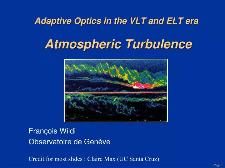
Adaptive Optics in the VLT and ELT era Atmospheric Turbulence. François Wildi Observatoire de Genève Credit for most slides : Claire Max (UC Santa Cruz). Atmospheric Turbulence Essentials.

E N D
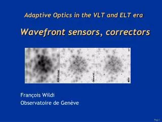
Adaptive Optics in the VLT and ELT era Atmospheric Turbulence François Wildi Observatoire de Genève Credit for most slides : Claire Max (UC Santa Cruz)
Atmospheric Turbulence Essentials • We, in astronomy, are essentially interested in the effect of the turbulence on the images that we take from the sky. This effect is to mix air masses of different index of refraction in a random fashion • The dominant locations for index of refraction fluctuations that affect astronomers are the atmospheric boundary layer , the tropopause and for most sites a layer in between (3-8km) where a shearing between layers occurs. • Atmospheric turbulence (mostly) obeys Kolmogorov statistics • Kolmogorov turbulence is derived from dimensional analysis (heat flux in = heat flux in turbulence) • Structure functions derived from Kolmogorov turbulence are r2/3
Fluctuations in index of refraction are due to temperature fluctuations • Refractivity of air where P = pressure in millibars, T = temp. in K, in microns n = index of refraction. Note VERY weak dependence on • Temperature fluctuations index fluctuations (pressure is constant, because velocities are highly sub-sonic. Pressure differences are rapidly smoothed out by sound wave propagation)
Turbulence arises in several places tropopause 10-12 km wind flow around dome boundary layer ~ 1 km stratosphere Heat sources w/in dome
When a mirror is warmer than dome air, convective equilibrium is reached. Remedies: Cool mirror itself, or blow air over it, improve mount Within dome: “mirror seeing” credit: M. Sarazin credit: M. Sarazin convective cells are bad To control mirror temperature: dome air conditioning (day), blow air on back (night)
Local “Seeing” -Flow pattern around a telescope dome Cartoon (M. Sarazin): wind is from left, strongest turbulence on right side of dome Computational fluid dynamics simulation (D. de Young) reproduces features of cartoon
Boundary layers: day and night • Wind speed must be zero at ground, must equal vwind several hundred meters up (in the “free” atmosphere) • Boundary layer is where the adjustment takes place, where the atmosphere feels strong influence of surface • Quite different between day and night • Daytime: boundary layer is thick (up to a km), dominated by convective plumes • Night-time: boundary layer collapses to a few hundred meters, is stably stratified. Perturbed if winds are high. • Night-time: Less total turbulence, but still the single largest contribution to “seeing”
Real shear generated turbulence (aka Kelvin-Helmholtz instability) measured by radar • Colors show intensity of radar return signal. • Radio waves are backscattered by the turbulence.
Kolmogorov turbulence, cartoon solar Outer scale L0 Inner scalel0 h Wind shear convection h ground
Kolmogorov turbulence, in words • Assume energy is added to system at largest scales - “outer scale” L0 • Then energy cascades from larger to smaller scales (turbulent eddies “break down” into smaller and smaller structures). • Size scales where this takes place: “Inertial range”. • Finally, eddy size becomes so small that it is subject to dissipation from viscosity. “Inner scale” l0 • L0 ranges from 10’s to 100’s of meters; l0 is a few mm
Assumptions of Kolmogorov turbulence theory Questionable • Medium is incompressible • External energy is input on largest scales (only), dissipated on smallest scales (only) • Smooth cascade • Valid only in inertial range L0 • Turbulence is • Homogeneous • Isotropic • In practice, Kolmogorov model works surprisingly well!
Concept Question • What do you think really determines the outer scale in the boundary layer? At the tropopause? • Hints:
Outer Scale ~ 15 - 30 m, from Generalized Seeing Monitor measurements • F. Martin et al. , Astron. Astrophys. Supp. v.144, p.39, June 2000 • http://www-astro.unice.fr/GSM/Missions.html
Atmospheric structure functions A structure function is measure of intensity of fluctuations of a random variable f (t) over a scale t : Df(t) = < [ f (t + t) - f ( t) ]2 > With the assumption that temperature fluctuations are carried around passively by the velocity field (for incompressible fluids), T and N have structure functions like • DT ( r ) = < [ T (x ) - v ( T + r ) ]2 > = CT2 r 2/3 • DN ( r ) = < [ N (x ) - N ( x + r ) ]2 > = CN2 r 2/3 CN2 is a “constant” that characterizes the strength of the variability of N. It varies with time and location. In particular, for a static location (i.e. a telescope) CN2 will vary with time and altitude
Typical values of CN2 10-14 • Index of refraction structure function DN ( r ) = < [ N (x ) - N ( x + r ) ]2 > = CN2 r 2/3 • Night-time boundary layer: CN2 ~ 10-13 - 10-15 m-2/3 Paranal, Chile, VLT
Turbulence profiles from SCIDAR Eight minute time period (C. Dainty, Imperial College) Starfire Optical Range, Albuquerque NM Siding Spring, Australia
Atmospheric Turbulence: Main Points • The dominant locations for index of refraction fluctuations that affect astronomers are the atmospheric boundary layer and the tropopause • Atmospheric turbulence (mostly) obeys Kolmogorov statistics • Kolmogorov turbulence is derived from dimensional analysis (heat flux in = heat flux in turbulence) • Structure functions derived from Kolmogorov turbulence are r2/3 • All else will follow from these points!
Definitions - Structure Function and Correlation Function • Structure function: Mean square difference • Covariance function: Spatial correlation of a random variable with itself
Relation between structure function and covariance function To derive this relationship, expand the product in the definition of D ( r ) and assume homogeneity to take the averages
Definitions - Spatial Coherence Function • Spatial coherence function of field is defined as Covariance for complex fn’s C (r) measures how “related” the field is at one position x to its values at neighboring positions x + r . Do not confuse the complex field with its phase f
Now evaluate spatial coherence function C (r) • For a Gaussian random variable with zero mean, • So • So finding spatial coherence function C (r) amounts to evaluating the structure function for phase D ( r ) !
Next solve for D ( r )in terms of the turbulence strength CN2 • We want to evaluate • Remember that
Solve for D ( r )in terms of the turbulence strength CN2, continued • But for a wave propagating vertically (in z direction) from height h to height h + h. This means that the phase is the product of the wave vector k (k=2p/l [radian/m]) x the Optical path Here n(x, z) is the index of refraction. • Hence
Solve for D ( r )in terms of the turbulence strength CN2, continued • Change variables: • Then Algebra…
Solve for D ( r )in terms of the turbulence strength CN2, continued • Now we can evaluate D ( r ) Algebra…
Solve for D ( r )in terms of the turbulence strength CN2, completed • But
Finally we can evaluate the spatial coherence function C (r) For a slant path you can add factor( sec )5/3 to account for dependence on zenith angle Concept Question: Note the scaling of the coherence function with separation, wavelength, turbulence strength. Think of a physical reason for each.
Given the spatial coherence function, calculate effect on telescope resolution • Define optical transfer functions of telescope, atmosphere • Definer0 as the telescope diameter where the two optical transfer functions are equal • Calculate expression for r0
Define optical transfer function (OTF) • Imaging in the presence of imperfect optics (or aberrations in atmosphere): in intensity units Image = Object Point Spread Function I = O PSF dx O(r - x) PSF( x ) • Take Fourier Transform: F( I ) = F(O )F( PSF ) • Optical Transfer Function is Fourier Transform of PSF: OTF = F( PSF ) convolved with
Examples of PSF’s and their Optical Transfer Functions Seeing limited OTF Seeing limited PSF Intensity -1 l / D l / r0 r0 / l D / l Diffraction limited PSF Diffraction limited OTF Intensity -1 l / r0 l / D D / l r0 / l
Now describe optical transfer function of the telescope in the presence of turbulence • OTF for the whole imaging system (telescope plus atmosphere) S ( f ) = B ( f ) T ( f ) Here B ( f ) is the optical transfer fn. of the atmosphere and T ( f) is the optical transfer fn. of the telescope (units of f are cycles per meter). f is often normalized to cycles per diffraction-limit angle (l / D). • Measure the resolving power of the imaging system by R = dfS ( f ) = dfB ( f ) T ( f )
Derivation of r0 • R of a perfect telescope with a purely circular aperture of (small) diameter d is R= df T ( f ) =( p / 4 ) ( d / l )2 (uses solution for diffraction from a circular aperture) • Define a circular aperture r0 such that the R of the telescope (without any turbulence) is equal to the R of the atmosphere alone: dfB ( f ) = dfT ( f ) ( p / 4 ) ( r0/ l )2
Derivation of r0 , continued • Now we have to evaluate the contribution of the atmosphere’s OTF: dfB ( f ) • B ( f ) = C ( l f ) (to go from cycles per meter to cycles per wavelength) Algebra…
Derivation of r0 , continued (6p / 5) G(6/5) K-6/5 • Now we need to do the integral in order to solve for r0 : ( p / 4 ) ( r0/ l )2 =dfB ( f ) = df exp (- K f 5/3) • Now solve for K: K = 3.44 (r0/ l )-5/3 B ( f ) = exp - 3.44 ( l f / r0 )5/3 = exp - 3.44 ( / r0 )5/3 Algebra… Replace by r
Scaling of r0 • r0is size of subaperture, sets scale of all AO correction • r0gets smaller when turbulence is strong (CN2 large) • r0gets bigger at longer wavelengths: AO is easier in the IR than with visible light • r0gets smaller quickly as telescope looks toward the horizon (larger zenith angles )
Typical values of r0 • Usually r0 is given at a 0.5 micron wavelength for reference purposes. It’s up to you to scale it by -1.2 to evaluate r0 at your favorite wavelength. • At excellent sites such as Paranal, r0 at 0.5 micron is 10 - 30 cm. But there is a big range from night to night, and at times also within a night. • r0 changes its value with a typical time constant of 5-10 minutes
Phase PSD, another important parameter • Using the Kolmogorov turbulence hypothesis, the atmospheric phase PSD can be derived and is • This expression canbeused to compute the amount of phase error over an uncorrectedpupil
Tip-tilt is single biggest contributor Focus, astigmatism, coma also big High-order terms go on and on…. Units: Radians of phase / (D / r0)5/6 Reference: Noll76