Download
1 / 15
160 likes | 599 Vues
13. The Weak Law and the Strong Law of Large Numbers. James Bernoulli proved the weak law of large numbers (WLLN) around 1700 which was published posthumously in 1713 in his treatise Ars Conjectandi. Poisson generalized Bernoulli’s theorem

E N D
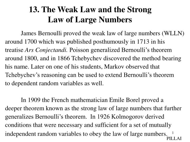
13. The Weak Law and the Strong Law of Large Numbers James Bernoulli proved the weak law of large numbers (WLLN) around 1700 which was published posthumously in 1713 in his treatise Ars Conjectandi. Poisson generalized Bernoulli’s theorem around 1800, and in 1866 Tchebychev discovered the method bearing his name. Later on one of his students, Markov observed that Tchebychev’s reasoning can be used to extend Bernoulli’s theorem to dependent random variables as well. In 1909 the French mathematician Emile Borel proved a deeper theorem known as the strong law of large numbers that further generalizes Bernoulli’s theorem. In 1926 Kolmogorov derived conditions that were necessary and sufficient for a set of mutually independent random variables to obey the law of large numbers. PILLAI
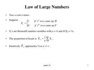
Let be independent, identically distributed Bernoulli random Variables such that and let represent the number of “successes” in n trials. Then the weak law due to Bernoulli states that [see Theorem 3-1, page 58, Text] i.e., the ratio “total number of successes to the total number of trials” tends to p in probability as n increases. A stronger version of this result due to Borel and Cantelli states that the above ratio k/n tends to p not only in probability, but with probability 1. This is the strong law of large numbers (SLLN). (13-1) PILLAI
What is the difference between the weak law and the strong law? The strong law of large numbers states that if is a sequence of positive numbers converging to zero, then From Borel-Cantelli lemma [see (2-69) Text], when (13-2) is satisfied the events can occur only for a finite number of indices n in an infinite sequence, or equivalently, the events occur infinitely often, i.e., the event k/n converges to palmost-surely. Proof: To prove (13-2), we proceed as follows. Since (13-2) PILLAI
we have and hence where By direct computation (13-3) PILLAI
since Substituting (13-4) also (13-3) we obtain Let so that the above integral reads and hence can coincide with j, k or l, and the second variable takes (n-1) values 0 (13-4) (13-5) PILLAI
thus proving the strong law by exhibiting a sequence of positive numbers that converges to zero and satisfies (13-2). We return back to the same question: “What is the difference between the weak law and the strong law?.” The weak law states that for every n that is large enough, the ratio is likely to be near p with certain probability that tends to 1 as n increases. However, it does not say that k/n is bound to stay near p if the number of trials is increased. Suppose (13-1) is satisfied for a given in a certain number of trials If additional trials are conducted beyond the weak law does not guarantee that the new k/n is bound to stay near p for such trials. In fact there can be events for which for in some regular manner. The probability for such an event is the sum of a large number of very small probabilities, and the weak law is unable to say anything specific about the convergence of that sum. However, the strong law states (through (13-2)) that not only all such sums converge, but the total number of all such events PILLAI
where is in fact finite! This implies that the probability of the events as n increases becomes and remains small, since with probability 1 only finitely many violations to the above inequality takes place as Interestingly, if it possible to arrive at the same conclusion using a powerful bound known as Bernstein’s inequality that is based on the WLLN. Bernstein’s inequality : Note that and for any this gives Thus PILLAI
Since for any real x, Substituting (13-7) into (13-6), we get But is minimum for and hence Similarly (13-6) (13-7) (13-8) PILLAI
and hence we obtain Bernstein’s inequality Bernstein’s inequality is more powerful than Tchebyshev’s inequality as it states that the chances for the relative frequency k /n exceeding its probability p tends to zero exponentially fast as Chebyshev’s inequality gives the probability of k /n to lie between and for a specific n. We can use Bernstein’s inequality to estimate the probability for k /n to lie between and for all large n. Towards this, let so that To compute the probability of the event note that its complement is given by (13-9) PILLAI
and using Eq. (2-68) Text, This gives or, Thus k /n is bound to stay near p for all large enough n, in probability, a conclusion already reached by the SLLN. Discussion: Let Thus if we toss a fair coin 1,000 times, from the weak law PILLAI
Thus on the average 39 out of 40 such events each with 1000 or more trials will satisfy the inequality or, it is quite possible that one out of 40 such events may not satisfy it. As a result if we continue the coin tossing experiment for an additional 1000 more trials, with k representing the total number of successes up to the current trial n, for it is quite possible that for few such n the above inequality may be violated. This is still consistent with the weak law, but “not so often” says the strong law. According to the strong law such violations can occur only a finite number of times each with a finite probability in an infinite sequence of trials, and hence almost always the above inequality will be satisfied, i.e., the sample space of k /n coincides with that of p as Next we look at an experiment to confirm the strong law: Example: 2n red cards and 2n black cards (all distinct) are shuffled together to form a single deck, and then split into half. What is the probability that each half will contain n red and n black cards?
Solution: From a deck of 4n cards, 2n cards can be chosen in different ways. To determine the number of favorable draws of n red and n black cards in each half, consider the unique draw consisting of 2n red cards and 2n black cards in each half. Among those 2n red cards, n of them can be chosen in different ways; similarly for each such draw there are ways of choosing n black cards.Thus the total number of favorable draws containing n red and n black cards in each half are among a total of draws. This gives the desired probability to be For large n, using Stingling’s formula we get PILLAI
For a full deck of 52 cards, we have which gives and for a partial deck of 20 cards (that contains 10 red and 10 black cards), we have and One summer afternoon, 20 cards (containing 10 red and 10 black cards) were given to a 5 year old child. The child split that partial deck into two equal halves and the outcome was declared a success if each half contained exactly 5 red and 5 black cards. With adult supervision (in terms of shuffling) the experiment was repeated 100 times that very same afternoon. The results are tabulated below in Table 13.1, and the relative frequency vs the number of trials plot in Fig 13.1 shows the convergence of k /n to p. PILLAI
Table 13.1 PILLAI
The figure below shows results of an experiment of 100 trials. 0.3437182 Fig 13.1