Download
1 / 29
990 likes | 2.62k Vues
Radial-Basis Function Networks. A function is radial basis (RBF) if its output depends on (is a non-increasing function of) the distance of the input from a given stored vector. RBFs represent local receptors, as illustrated below, where each green point is a stored vector used in one RBF.

E N D
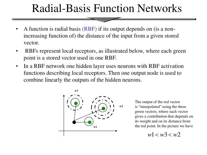
Radial-Basis Function Networks • A function is radial basis(RBF) if its output depends on (is a non-increasing function of) the distance of the input from a given stored vector. • RBFs represent local receptors, as illustrated below, where each green point is a stored vector used in one RBF. • In a RBF network one hidden layer uses neurons with RBF activation functions describing local receptors. Then one outputnode is used to combine linearly the outputs of the hidden neurons. w3 The output of the red vector is “interpolated” using the three green vectors, where each vector gives a contribution that depends on its weight and on its distance from the red point. In the picture we have w2 w1
x1 w1 x2 y wm1 xm RBF ARCHITECTURE • One hidden layer with RBF activation functions • Output layer with linear activation function.
HIDDEN NEURON MODEL • Hidden units: use radial basis functions the output depends on the distance of the input x from the center t φ( || x - t||) x1 φ( || x - t||) t is called center is called spread center and spread are parameters x2 xm
Hidden Neurons • A hidden neuron is more sensitive to data points near its center. • For Gaussian RBF this sensitivity may be tuned by adjusting the spread , where a larger spread impliesless sensitivity. • Biological example: cochlear stereocilia cells (in our ears ...) have locally tuned frequency responses.
center Small Large Gaussian RBF φ φ : is a measure of how spread the curve is:
Types of φ • Multiquadrics: • Inversemultiquadrics: • Gaussianfunctions (most used):
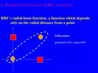
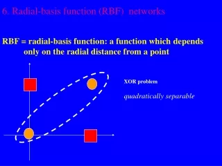
x2 (0,1) (1,1) 0 1 y x1 (0,0) (1,0) Example: the XOR problem • Input space: • Output space: • Construct an RBF pattern classifier such that: (0,0) and (1,1) are mapped to 0, class C1 (1,0) and (0,1) are mapped to 1, class C2
φ2 (0,0) Decision boundary 1.0 0.5 (1,1) 1.0 φ1 0.5 (0,1) and (1,0) Example: the XOR problem • In the feature (hidden layer) space: • When mapped into the feature space < 1 , 2 > (hidden layer), C1 and C2become linearly separable. Soa linear classifier with 1(x) and 2(x) as inputs can be used to solve the XOR problem.
x1 t1 -1 y x2 t2 -1 +1 RBF NN for the XOR problem
RBF network parameters • What do we have to learn for a RBF NN with a given architecture? • The centersof theRBF activation functions • the spreads of the Gaussian RBF activation functions • the weights from the hidden to the output layer • Different learning algorithms may be used for learning the RBF network parameters. We describe three possible methods for learning centers, spreads and weights.
Learning Algorithm 1 • Centers: are selected at random • centers are chosen randomly from the training set • Spreads: are chosen by normalization: • Then the activation function of hidden neuron becomes:
Learning Algorithm 1 • Weights:are computed by means of the pseudo-inverse method. • For an example consider the output of the network • We would like for each example, that is
Learning Algorithm 1 • This can be re-written in matrix form for one example and for all the examples at the same time
Learning Algorithm 1 let then we can write If is the pseudo-inverse of the matrix we obtain the weights using the following formula
Learning Algorithm 2: Centers • clustering algorithm for finding the centers • Initialization: tk(0) random k = 1, …, m1 • Sampling: draw x from input space • Similaritymatching: find index of center closer to x • Updating: adjust centers • Continuation: increment n by 1, goto 2 and continue until no noticeable changes of centers occur
Learning Algorithm 2: summary • Hybrid Learning Process: • Clustering for finding the centers. • Spreads chosen by normalization. • LMS algorithm (see Adaline) for finding the weights.
Learning Algorithm 3 • Apply the gradient descent method for finding centers, spread and weights, by minimizing the (instantaneous) squared error • Update for: centers spread weights
Comparison with FF NN RBF-Networks are used for regression and for performing complex (non-linear) pattern classification tasks. Comparison between RBFnetworks and FFNN: • Both are examples of non-linear layered feed-forward networks. • Both are universal approximators.
Comparison with multilayer NN • Architecture: • RBF networks have one single hidden layer. • FFNN networks may have more hidden layers. • Neuron Model: • In RBF the neuron model of the hidden neurons is different from the one of the output nodes. • Typically in FFNN hidden and output neurons share a common neuron model. • The hidden layer of RBF is non-linear, the output layer of RBF is linear. • Hidden and output layers of FFNN are usually non-linear.
Comparison with multilayer NN • Activation functions: • The argument of activation function of each hidden neuron in a RBF NN computes the Euclidean distance between input vector and the center of that unit. • The argument of the activation function of each hidden neuron in a FFNN computes the inner product of input vector and the synaptic weight vector of that neuron. • Approximation: • RBF NN using Gaussian functions construct local approximations to non-linear I/O mapping. • FF NN construct global approximations to non-linear I/O mapping.
Application: FACE RECOGNITION • The problem: • Face recognition of persons of a known group in an indoor environment. • The approach: • Learn face classes over a wide range of poses using an RBF network.
Dataset • database • 100 images of 10 people (8-bit grayscale, resolution 384 x 287) • for each individual, 10 images of head in different pose from face-on to profile • Designed to asses performance of face recognition techniques when pose variations occur
Datasets All ten images for classes 0-3 from the Sussex database, nose-centred and subsampled to 25x25 before preprocessing
Approach: Face unit RBF • A face recognition unit RBF neural networks is trained to recognize a single person. • Training uses examples of images of the person to be recognized as positive evidence, together with selected confusable images of other people as negative evidence.
Network Architecture • Input layer contains 25*25 inputs which represent the pixel intensities (normalized) of an image. • Hidden layer contains p+a neurons: • p hidden pro neurons (receptors for positive evidence) • ahidden anti neurons (receptors for negative evidence) • Output layer contains two neurons: • One for the particular person. • One for all the others. The output is discarded if the absolute difference of the two output neurons is smaller than a parameter R.
RBF Architecture for one face recognition Output units Linear Supervised RBF units Non-linear Unsupervised Input units
Hidden Layer • Hidden nodes can be: • Pro neurons: Evidence for that person. • Anti neurons: Negative evidence. • The number of pro neurons is equal to the positive examples of the training set. For each pro neuron there is either one or two anti neurons. • Hidden neuron model: Gaussian RBF function.
Training and Testing • Centers: • of a pro neuron: the corresponding positive example • of an anti neuron: the negative example which is most similar to the corresponding pro neuron, with respect to the Euclidean distance. • Spread: average distance of the center from all other centers. So the spread of a hidden neuron n is where H is the number of hidden neurons and is the center of neuron . • Weights: determined using the pseudo-inverse method. • A RBF network with 6 pro neurons, 12 anti neurons, and R equal to 0.3, discarded 23 pro cent of the images of the test set and classified correctly 96 pro cent of the non discarded images.