Download
1 / 47
470 likes | 673 Vues
Synaptic Dynamics: Unsupervised Learning. Part Ⅱ Wang Xiumei. 1. Stochastic unsupervised learning and stochastic equilibrium; 2. Signal Hebbian Learning; 3. Competitive Learning. 1.Stochastic unsupervised learning and stochastic equilibrium. ⑴ The noisy random unsupervised

E N D
Synaptic Dynamics:Unsupervised Learning Part Ⅱ Wang Xiumei
1.Stochastic unsupervised learning and stochastic equilibrium; 2.Signal Hebbian Learning; 3.Competitive Learning.
1.Stochastic unsupervised learning and stochastic equilibrium ⑴ The noisy random unsupervised learning law; ⑵ Stochastic equilibrium; ⑶ The random competitive learning law; ⑷ The learning vector quantization system.
The noisy random unsupervised learning law The random-signal Hebbian learning law: (4-92) denotes a Browian-motion diffusion process, each term in (4-92)demotes a separate random process.
The noisy random unsupervised learning law • Using noise relationship: we can rewrite (4-92): (4-93) We assume the zero-mean, Gaussian white-noise process ,and use equation :
The noisy random unsupervised learning law We can get a noisy random unsupervised learning law (4-94) Lemma: (4-95) is finite variance. proof: P132
The noisy random unsupervised learning law The lemma implies two points: 1, stochastic synapses vibrate in equilibrium, and they vibrate at least as much as the driving noise process vibrates; 2,the synaptic vector changes or vibrate at every instant t, and equals a constant value. wanders in a brownian motion about the constant value E[ ].
Stochastic equilibrium When synaptic vector stops moving, synaptic equilibrium occurs in “steady state”, (4-101) synaptic vector reaches synaptic equilibrium when only the random noise vector change : (4-103)
The random competitive learning law The random competitive learning law The random linear competitive learning law
The self-organizing map system • The self-organizing map system equations:
The self-organizing map system The self-organizing map is a unsupervised clustering algorithm. Compared with traditional clustering algorithms, its centroid can be mapped a curve or plain, and it remains topological structure.
2.Signal HebbianLearning ⑴Recency effects and forgetting; ⑵Asymptotic correlation encoding; ⑶Hebbian correlation decoding.
Signal Hebbian Learning The deterministic first-order signal Hebbian learning law: (4-132) (4-133)
Recency effects and forgetting Hebbian synapses learn an exponentially weighted average of sampled patterns. the forgetting term is . The simplest local unsupervised learning law:
Asymptotic correlation encoding The synaptic matrix of long-term memory tracesasymptotically approaches the bipolar correlation matrix : X and Y denotes the bipolar signal vectors and .
Asymptotic correlation encoding In practice we use a diagonal fading-memory exponential matrix W compensates for the inherent exponential decay of learned information: (4-142)
Hebbian correlation decoding First we consider the bipolar correlation encoding of theM bipolar associations ,and turn bipolar associations into binary vector associations . replace -1s with 0s
Hebbian correlation decoding The Hebbian encoding of the bipolar associations corresponds to the weighted Hebbian encoding scheme if the weight matrix W equals the (4-143)
Hebbian correlation decoding We use the Hebbian synaptic M for bidirectional processing of and neuronal signals, and pass neural signal through M in the forward direction, in the backward direction.
Hebbian correlation decoding Signal-noise decomposition:
Hebbian correlation decoding Correction coefficients : (4-149) They can make each vector resemble in sign as much as possible. The same correction property holds in the backward direction .
Hebbian correlation decoding We definethe Hamming distance between binary vectors and
Hebbian correlation decoding [number of common bits] -[number of different bits ]
Hebbian correlation decoding • Suppose binary vector is close to , Then ,geometrically, the two patterns are less than half their space away from each other, So . In the extreme case ;so . • The rare case that result in , and the correction coefficients should be discarded.
Hebbian correlation decoding 3) Suppose is far away from , . In the extreme case: , .
binary vector bipolar vector sum contiguous correlation -encoded associations: Hebbian encoding method T
Hebbian encoding method Example(P144): consider the three-step limit cycle: convert bit vectors to bipolar vectors:
Hebbian encoding method Produce the asymmetric TAM matrix T:
Hebbian encoding method Passing the bit vectors through T in the forward direction produces: Produce the forward limit cycle:
Competitive Learning The deterministic competitive learning law: (4-165) (4-166) We see that the competitive learning law uses the nonlinear forgetting term: .
Competitive Learning Heb learning law uses the linear forgetting term . So the two laws differ in how they forget, not in how they learn. In both cases when -when the jth competing neuron wins-the synaptic value encodes the forcing signal and encodes it exponentially quickly.
3.Competitive Learning. ⑴ Competition as Indication; ⑵ Competition as correlation detection; ⑶ Asymptotic centroid estimation; ⑷ Competitive covariance estimation.
Competition as indication Centroid estimation requires that the competitive signal approximate the indicator function of the locally sampled pattern class : (4-168)
Competition as indication If sample pattern X comes from region , the jth competing neuron in should win, and all other competing neurons should Lose. In practice we usually use the random linear competitive learning law and a simple additive model. (4-169)
Competition as indication the inhibitive-feedback term equals the additive sum of synapse-weighted signal: (4-170) if the jth neuron wins, and to if instead the kth neuron wins.
Competition as correlation detection The metrical indicator function: (4-171) If the input vector X is closer to synaptic vector than to all other stored synaptic vectors, the jth competing neuron will win.
Competition as correlation detection Using equinorm property, we can get the equivalent equalities(P147): (4-174) (4-178) (4-179)
Competition as correlation detection From the above equality, we can get: The jth Competing neuron wins iff the input signal or pattern correlates maximally with . The cosine law: (4-180)
Asymptotic centroid estimation The simpler competitive law: (4-181) If we use the equilibrium condition: (4-182)
Asymptotic centroid estimation Solving for the equilibrium synaptic vector: (4-186) It show that equals the centroid of .
Competitive covariance estimation Centroids provides a first-order Estimate of how the unknown probability Density function behaves in the regions , and local covariances provide a second-order description.
Competitive covariance estimation Extend the competitive learning laws to asymptotically estimate the local conditional covariance matrices : (4-187) (4-189) denotes the centriod.
Competitive covariance estimation The fundamental theorem of estimation theory [Mendel 1987]: (4-190) is Borel-measurable random vector function
Competitive covariance estimation At each iteration we estimate the unknown centroid as the current synaptic vector ,In this sense becomes an error conditional covariance matrix . the stochastic difference-equation algorithm: (4-191-192)
Competitive covariance estimation denotes an appropriately decreasing sequence of learning coefficients in(4-192). If the ith neuron loses the metrical competition
Competitive covariance estimation The algorithm(4-192) corresponds to the stochastic differential equation: (4-195) (4-199)