Download
1 / 22
230 likes | 372 Vues
Parallel Graphics Rendering. Matthew Campbell Senior, Computer Science mcampbel@vt.edu. Overview. Motivation Three categories of parallel rendering Our approach Results Questions. Motivation. PC graphics cards are getting faster at an exponential rate.

E N D
Parallel Graphics Rendering Matthew Campbell Senior, Computer Science mcampbel@vt.edu
Overview • Motivation • Three categories of parallel rendering • Our approach • Results • Questions
Motivation • PC graphics cards are getting faster at an exponential rate. • PC graphics boards are much cheaper than proprietary SGI hardware. • Geforce4 FX = $150.00 (130 Mtris/sec) • SGI Onyx 300 = $145,000 (80 Mtris/sec) • Maintanance costs are lower • Replacement parts are easy to get. • PC’s are not as complicated as proprietary hardware.
Parallel Rendering • String together numerous PC’s with good graphics boards and render the models in parallel. • Increased performace • Better technology tracking • Three groups of algorithms: • Sort-First • Sort-Middle • Sort-Last
Rendering Pipeline • Transformation stage: • Per-Vertex operations • Primitive Assembly • 3D World Space! • Rasterization stage: • Per-fragment operations • Texture mapping • 2D Image Space!
Parallel Rendering – Sort Last • Sort Last • Distribute polygons • Round robin distribution resulting in an equal load on each processor. • Pass through entire rendering pipeline. • Transformation / Rasterization (see last slide) • Each CPU now has the entire scene • But individual scenes are incomplete • Hidden polygons may be visible • Solution: Image composition
Sort Last – Image Composition • The scene at each CPU has a frame buffer with color values for each pixel and a depth buffer with Z values for each pixel. • Composition: Given 2 scenes it computes the color of the pixel at each screen coordinate • Compare the depth buffer values at each pixel location. The resultant color value is the color of the pixel corresponding to a lower z axis value. • Alpha blending is more complex. • Why?
Sort Last – Image Composition • Time complexity of the previous sort algorithm is O(n), which is pretty bad. • Can we improve it? • Alternate algorithms: • Tree composition. • Rotating rings. • Binary composition.
Sort-Last Performance • Sort-Last has very high communication bandwidth requirement. • Each processor needs to send and receive an entire frame • 1280x1024 resolution, 24-bits for color, 16-bits for depth, 30fps • = (3.9MB + 2.6MB) * 30 = 196MB/sec bidirectional! • Need a very fast network interconnecting the CPUs in the cluster. • In actuality, we need more bandwidth, because we haven’t taken into account, the time it takes to render the scene! • But.. No overhead for rendering the actual scene!
Parallel Rendering – Sort Middle • Sort Middle • Distribute polygons in a round robin fashion • Trap polygons between geometry and rasterization phases • Each CPU in the cluster is responsible for a specific region in screen coordinates • Calculate the bounding boxes (screen space) for the trapped polygons and redistribute them to the appropriate CPU responsible for the region. • Collate Images
Parallel Rendering – Sort Middle • How do you divide the screen into regions? • Strips (either horizontal or vertical) • Squares • What is the mapping ratio between CPUs and regions? • One-to-One: Each CPU manages 1 region • One-to-Many: Each CPU manages many regions • What about polygons that cross region boundaries? • Multiple CPUs render the same polygon.
Sort-Middle Performance • Load-balancing can be poor. The slowest CPU will block the system from rendering the next scene. • Load balancing is highly scene and view dependent. • Need adaptive load-balancing schemes. • In high polygon count scenes, the size of each polygon can be very small (~1 – 2 pixels). • In this case, sort middle requires more bandwidth than sort-last. • Communication bandwidth required is dependent on the scene complexity. (Bad)
Parallel Rendering – Sort First • Sort First • Distribute polygons round-robin to all CPUs. • Calculate bounding volumes for each polygon • Remember, we are still in the world coordinate system. • Each CPU is responsible for 1 volume. • Redistribute polygons based on bounding volumes. • Pass through complete rendering pipeline • In the end we have sub-images at each processor. • Designate a coordinator node, which receives sub-images from all other processors. • Coordinator collates sub-images into the final image.
Sort First - Performance • Communication bandwidth required is based only on screen space resolution. • Example: • 4 CPUs, 1024*1024 scene, 32 bits/color • The coordinator node receives 1024*1024*24 bits/frame. ~ 3MB. • Bandwidth: 90MB/sec for 30 fps. • Problem: Similar to sort-middle, load balancing is scene dependent. • Bigger issue: Can’t use a one-to-many CPU to region mapping. • Or can you?
Parallel Rendering Issues • Cannot break the rendering pipeline • Pipeline is implemented in hardware • Therefore, very expensive. Could lead to excessive stalls, cache misses, etc.. • Modern graphics cards have large amounts of memory on the board and much faster access times. • 8GB/sec vs. 1GB/sec for AGP4x • Graphics driver source code is unavailable • Additional cost/overhead due to framebuffer accesses.
Our Approach • High Performance real-time rendering. • High scene complexity and/or multiple displays as in a VE. • Target: 200-300 million triangles/sec. In comparison the best SGI platform – Reality Monster is capable of 80 million polygons/sec • Approach: • Distributed Sort-First. • Two level sorting. • Organize your model in a spatial tree data structure. • At run-time compare bounding volumes for interior nodes of the tree. The bounding volume for an interior node is a superset of its children. This minimizes comparisons. • Fine pruning based on viewing frustum.
Hardware • 32 Intel Xeon processor cluster (1.5 GHz processor) • 256 MB RDRAM/node (3.2 GB/sec memory bandwidth) • Myrinet (4 Gbps) and Fast Ethernet (200 Mbps full-duplex) communication fabrics. • 64 bit/66 MHz PCI bus (4 Gbps throughput) • 4x AGP (1GB/sec throughput)
Software • Extensible Parallel 3D Rendering Engine • Supports large geometric databases, including standard formats such as 3D Studio • Provides an extensible API. • Underlying system is based on OpenGL. • Based on dynamic shared object model. • Dynamic Load Balancing • Adaptively resizes volumes assigned to a processor for single display systems. • Adaptively changes the number of processors and rendering volumes for multi-display systems.
Software Architecture • Master-Slave arrangement • Multi-threaded • Two stage parallel rendering pipeline.
Results – Rendering Rate Figure 1:Scalability of our implementation. Actual depicts the performance taking into account triangle overlap among nodes, effective depicts what the system is capable of delivering. Left image uses a real world dataset (LIDAR data). Right image uses a generated dataset to fully exploit the overlap issue.
Results – Load Balancing Figure 2: The effects of load balancing on 4 nodes (left) and 16 nodes (right). The graph depicts the individiual frame times for first 100 frames.