Download
1 / 49
500 likes | 645 Vues
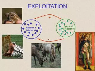
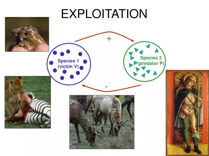
+. Species 2 (predator P). Species 1 (victim V). -. EXPLOITATION. Classic predation theory is built upon the idea of time constraint (foraging theory): A 24 hour day is divided into time spent unrelated to eating: social interactions mating rituals grooming sleeping

E N D
+ Species 2 (predator P) Species 1 (victim V) - EXPLOITATION
Classic predation theory is built upon the idea of time constraint (foraging theory): • A 24 hour day is divided into time spent unrelated to eating: • social interactions • mating rituals • grooming • sleeping • And eating-related activities: • searching for prey • pursuing prey • subduing the prey • eating the prey • digesting (may not always exclude other activities)
The time constraints on foraging Foraging time other essential activities foraging
The time constraints on foraging Foraging time other essential activities Handling time Search time search handling
Search time: all activities up to the point of spotting the prey • searching • Handling time: all activities from spotting to digesting the prey • pursuing • subduing, killing • eating • (transporting, burying, regurgitating, etc) • digesting • Caveat: not all activities may be mutually exclusive • ex. Digesting and non-eating related activities
The time constraints on foraging Foraging time other essential activities Handling time Search time eating search pursuing & subduing eating time pursuit & subdue time
Filter feeder: Sit & wait predator (spider) eating waiting eating digesting subduing Different species will allocate foraging time differently:
Well-fed mammalian predator: Starving mammalian Predator (victims at low dnsity): eating eating searching pursuing & subduing pursuing & subduing searching Time allocation also depends on victim density and predator status:
Total search time per day Total handing time per day Total foraging time is fixed (or cannot exceed a certain limit). C.S. (Buzz) Holling The math of predation: (After C.S. Holling)
1) Define the per-predator capture rate as the number of victims captured (n) per time spent searching (ts): 2) Capture rate is a function of victim density (V). Define a as capture efficiency. 3) Every captured victim requires a certain time for “processing”.
n/t = capture rate
Capture rate limited by predator’s handling time. Capture rate Capture rate limited by prey density and capture efficiency Prey density (V)
nymph Damselfly (Thompson 1975)
Asymptote: 1/h Decreasing prey size The larger the prey, the greater the handling time. (Thompson 1975)
Three Functional Responses (of predators with respect to prey abundance): Holling Type I: Consumption per predator depends only on capture efficiency: no handling time constraint. Holling Type II: Predator is constrained by handling time. Holling Type III: Predator is constrained by handling time but also changes foraging behavior when victim density is low.
Type I: Type II Type III Type I (filter feeders) Type II (predator with significant handling time limitations) Per predator consumption rate Type III (predator who pays less attention to victims at low density) victim density
Thin algae suspension culture Daphnia path Thick algae suspension culture Holling Type I functional response: Type I functional response Daphnia (Filter feeder on microscopic freshwater organism)
Holling Type II functional response: Slug eating grass Cattle grazing in sagebrush grassland
Holling Type III functional response: Paper wasp, a generalist predator, eating shield beetle larvae: The wasp learns to hunt for other prey, when the beetle larvae becomes scarce.
The dynamics of predator prey systems are often quite complex and dependent on foraging mechanics and constraints.
Gause’s Predation Experiments: Didinium nasutumeatsParamecium caudatum:
Paramecium in oat medium: • logistic growth. 2) Paramecium with Didinium in oat medium: extinction of both. 3) Paramecium with Didinium in oat medium with sediment: extinction of Didinium. Gause’s Predation Experiments:
Greenhouse whitefly Parasitoid wasp A fly and its wasp predator: Laboratory experiment (Burnett 1959)
spider mite on its own with predator in simple habitat Spider mites with predator in complex habitat (Laboratory experiment) Predatory mite (Huffaker 1958)
Azuki bean weevil and parasitoid wasp (Laboratory experiment) (Utida 1957)
collared lemming stoat (Greenland) lemming stoat (Gilg et al. 2003)
prey boom predator boom Predator bust prey bust Possible outcomes of predator-prey interactions: • The predator goes extinct. • Both species go extinct. • Predator and prey cycle: • Predator and prey coexist in stable ratios.
Putting together the population dynamics: Predators (P): Victim consumption rate * Victim Predator conversion efficiency - Predator death rate Victims (V): Victim renewal rate – Victim consumption rate
Choices, choices…. • Victim growth assumption: • exponential • logistic • Functional response of the predator: • always proportional to victim density (Holling Type I) • Saturating (Holling Type II) • Saturating with threshold effects (Holling Type III)
The simplest predator-prey model (Lotka-Volterra predation model) Exponential victim growth in the absence of predators. Capture rate proportional to victim density (Holling Type I).
Predator density Victim isocline: Predator isocline: Victim density
Predator density Victim isocline: Predator isocline: Victim density dV/dt < 0 dP/dt < 0 dV/dt < 0 dP/dt > 0 dV/dt > 0 dP/dt > 0 dV/dt > 0 dP/dt < 0 Show me dynamics
Predator density Victim isocline: Predator isocline: Victim density
Predator density Victim isocline: Preator isocline: Victim density
Predator density Victim isocline: Preator isocline: Victim density Neutrally stable cycles! Every new starting point has its own cycle, except the equilibrium point. The equilibrium is also neutrally stable.
Logistic victim growth in the absence of predators. Capture rate proportional to victim density (Holling Type I).
r a r c Predator density Victim density Predator isocline: Victim isocline:
P V Stable Point ! Predator and Prey cycle move towards the equilibrium with damping oscillations.
Exponential growth in the absence of predators. Capture rate Holling Type II (victim saturation).
r kD Predator density Victim density Victim isocline: Predator isocline:
Unstable Equilibrium Point! Predator and prey move away from equilibrium with growing oscillations. P V
No density-dependence in either victim or prey (unrealistic model, but shows the propensity of PP systems to cycle): P V P Intraspecific competition in prey: (prey competition stabilizes PP dynamics) V P Intraspecific mutualism in prey (through a type II functional response): V
Predators population growth rate (with type II funct. resp.): Victim population growth rate (with type II funct. resp.):
Predator density Predator isocline: Victim isocline: Victim density Rosenzweig-MacArthur Model
Predator density Predator isocline: Victim isocline: Victim density Rosenzweig-MacArthur Model If the predator needs high victim density to survive, competition between victims is strong, stabilizing the equilibrium!
Predator density Predator isocline: Victim isocline: Victim density Rosenzweig-MacArthur Model If the predator drives the victim population to very low density, the equilibrium is unstable because of strong mutualistic victim interactions.
Predator density Predator isocline: Victim isocline: Victim density Rosenzweig-MacArthur Model However, there is a stable PP cycle. Predator and prey still coexist!
The Rosenzweig-MacArthur Model illustrates how the variety of outcomes in Predator-Prey systems can come about: • Both predator and prey can go extinct if the predator is too efficient capturing prey (or the prey is too good at getting away). • The predator can go extinct while the prey survives, if the predator is not efficient enough: even with the prey is at carrying capacity, the predator cannot capture enough prey to persist. • With the capture efficiency in balance, predator and prey can coexist. • a) coexistence without cyclical dynamics, if the predator is relatively inefficient and prey remains close to carrying capacity. • b) coexistence with predator-prey cycles, if the predators are more efficient and regularly bring victim densities down below the level that predators need to maintain their population size.