Download
1 / 16
160 likes | 268 Vues
LU Decomposition. Greg Beckham, Michael Sedivy. Overview. Step 1. This is handled implicitly in the code by only calculating the diagonal for β. Step 2. Calculating β ij. for(j = 0; j < n; j++) // This is the loop over columns of Crout's method {

E N D
LU Decomposition Greg Beckham, Michael Sedivy
Step 1 This is handled implicitly in the code by only calculating the diagonal for β
Calculating βij for(j = 0; j < n; j++) // This is the loop over columns of Crout's method { for(i = 0; i < j; i++) // Equation (2.3.12) except for i = j { sum = a[i][j]; for(k = 0; k < i; k++) sum -= a[i][k] * a[k][j]; a[i][j] = sum; } … }
for(j = 0; j < n; j++) // This is the loop over columns of Crout's method { … for(i = j; i < n; i++)// This is i=j of equation (2.3.12) and i=j+1 { // N-1 of equation (2.3.13) sum = a[i][j]; for(k = 0; k < j; k++) sum -= a[i][k] * a[k][j]; a[i][j] = sum; … } … if(j != n - 1) // Divide by the pivot element { dum = 1.0/(a[j][j]); for(i = j + 1; i < n; i++) a[i][j] *= dum; } … }
Pivoting • Initially finds largest element in each row • Used as a “scaling factor”, not sure of use other than to rollover for(i = 0; i < n; i++) // Loop over the rows to get implicit scaling { // information big = 0.0; for(j = 0; j < n; j++) { if((temp = fabs(a[i][j])) > big) big = temp; } if (big == 0.0) { printf("ERROR: Singular matrix\n"); } // non-zero largest element. vv[i] = 1.0/big; // Save the scaling }
Pivoting • Finds maximum if((dum = vv[i] * fabs(sum)) >= big) { // Is the figure of merit for the pivot better than the best so far? big = dum; imax = i; }
Pivoting • Performs row interchanges if(j != imax) // Do we need to interchange rows? { for(k = 0; k < n; k++) // Interchange rows { dum = a[imax][k]; a[imax][k] = a[j][k]; a[j][k] = dum; } d = -d; // change the parity of d vv[imax] = vv[j]; // interchange scale factor } indx[j] = imax;
Related Questions • What is the advantage of LU(P) solver over GJ(P) solver? (Complexity) • Both are O(N3) • After LU(P) is solved, more solutions supposed to be found in O (N2) • Are you keeping L and U in the same matrix, or separate? Advantage/disadvantage? • LU are being created in place in the same matrix. • The advantage to this strategy is lower memory usage • The disadvantage is that the original matrix is lost • I am somewhat confused with extraction of P in decomposition, and how it is then used in eq solving. Can you elaborate more?
Related Questions • Cormen et al., p 824, used a single array instead of P. Needs careful explanation. • From Cormen et al. 825. “we dynamically maintain the permutation matrix P as an array π, where π[i] = j means that the ith row of P contains a 1 in column j |2| | 0 1 0 | π = |3| => P | 0 0 1 | |1| | 1 0 0 |
Related Questions • How complex equations are solved? (in Text) • If only the right hand side vector is complex then the operation can be performed by solving for the real part, then the imaginary • If the matrix itself is complex then • Rewrite the algorithm for complex values • Split the real and imaginary parts into separate real number and solve using existing algorithm • A * x – C * y = b • C * x + A * y = b
GJ vs. LUP Average Difference is 2.765471 Average Difference is 1.255924