Download
1 / 41
410 likes | 796 Vues
Graph Clustering. Why graph clustering is useful?. Distance matrices are graphs as useful as any other clustering Identification of communities in social networks Webpage clustering for better data management of web data. Outline. Min s-t cut problem Min cut problem Multiway cut

E N D
Why graph clustering is useful? • Distance matrices are graphs as useful as any other clustering • Identification of communities in social networks • Webpage clustering for better data management of web data
Outline • Min s-t cut problem • Min cut problem • Multiway cut • Minimum k-cut • Other normalized cuts and spectral graph partitionings
Min s-t cut • Weighted graph G(V,E) • An s-t cut C = (S,T) of a graph G = (V, E) is a cut partition of V into S and T such thats∈S and t∈T • Cost of a cut: Cost(C) = Σe(u,v) uЄS, v ЄT w(e) • Problem:Given G, s and t find the minimum cost s-t cut
Max flow problem • Flow network • Abstraction for material flowing through the edges • G = (V,E) directed graph with no parallel edges • Two distinguished nodes: s = source, t= sink • c(e) = capacity of edge e
Cuts • An s-t cut is a partition (S,T) of V with sЄS and tЄT • capacity of a cut (S,T) is cap(S,T) = Σe out of Sc(e) • Find s-t cut with the minimum capacity: this problem can be solved optimally in polynomial time by using flow techniques
Flows • An s-t flow is a function that satisfies • For each eЄE 0≤f(e) ≤c(e) [capacity] • For each vЄV-{s,t}: Σe in to vf(e) = Σe out ofvf(e) [conservation] • The value of a flow f is: v(f) = Σe out of s f(e)
Max flow problem • Find s-t flow of maximum value
Flows and cuts • Flow value lemma: Let f be any flow and let (S,T) be any s-t cut. Then, the net flow sent across the cut is equal to the amount leaving s Σe out ofS f(e) – Σe in toS f(e) = v(f)
Flows and cuts • Weak duality: Let f be any flow and let (S,T) be any s-t cut. Then the value of the flow is at most the capacity of the cut defined by (S,T): v(f) ≤cap(S,T)
Certificate of optimality • Let f be any flow and let (S,T) be any cut. If v(f)= cap(S,T) then f is a max flow and (S,T) is a min cut. • The min-cut max-flow problems can be solved optimally in polynomial time!
Setting • Connected, undirected graph G=(V,E) • Assignment of weights to edges: w: ER+ • Cut: Partition of V into two sets: V’, V-V’. The set of edges with one end point in V and the other in V’ define the cut • The removal of the cut disconnects G • Cost of a cut: sum of the weights of the edges that have one of their end point in V’ and the other in V-V’
Min cut problem • Can we solve the min-cut problem using an algorithm for s-t cut?
Randomized min-cut algorithm • Repeat : pick an edge uniformly at random and merge the two vertices at its end-points • If as a result there are several edges between some pairs of (newly-formed) vertices retain them all • Edges between vertices that are merged are removed (no self-loops) • Until only two vertices remain • The set of edges between these two vertices is a cut in G and is output as a candidate min-cut
Observations on the algorithm • Every cut in the graph at any intermediate stage is a cut in the original graph
Analysis of the algorithm • C the min-cut of size k G has at least kn/2 edges • Why? • Ei: the event of not picking an edge of C at the i-th step for 1≤i ≤n-2 • Step 1: • Probability that the edge randomly chosen is in Cis at most 2k/(kn)=2/n Pr(E1) ≥ 1-2/n • Step 2: • If E1occurs, then there are at least n(n-1)/2 edges remaining • The probability of picking one from C is at most 2/(n-1) Pr(E2|E1) = 1 – 2/(n-1) • Step i: • Number of remaining vertices: n-i+1 • Number of remaining edges: k(n-i+1)/2 (since we never picked an edge from the cut) • Pr(Ei|Πj=1…i-1Ej) ≥ 1 – 2/(n-i+1) • Probability that no edge in C is ever picked: Pr(Πi=1…n-2Ei) ≥ Πi=1…n-2(1-2/(n-i+1))=2/(n2-n) • The probability of discovering a particular min-cut is larger than 2/n2 • Repeat the above algorithm n2/2 times. The probability that a min-cut is not found is (1-2/n2)n^2/2 < 1/e
Multiway cut (analogue of s-t cut) • Problem: Given a set of terminals S = {s1,…,sk} subset of V, a multiway cut is a set of edges whose removal disconnects the terminals from each other. The multiway cut problem asks for the minimum weight such set. • The multiway cut problem is NP-hard (for k>2)
Algorithm for multiway cut • For each i=1,…,k, compute the minimum weight isolating cut for si, say Ci • Discard the heaviest of these cuts and output the union of the rest, say C • Isolating cut forsi: The set of edges whose removal disconnects sifrom the rest of the terminals • How can we find a minimum-weight isolating cut? • Can we do it with a single s-t cut computation?
Approximation result • The previous algorithm achieves an approximation guarantee of 2-2/k • Proof
Minimum k-cut • A set of edges whose removal leaves k connected components is called a k-cut. The minimum k-cut problem asks for a minimum-weightk-cut • Recursively compute cuts in G (and the resulting connected components) until there are k components left • This is a (2-2/k)-approximation algorithm
Minimum k-cut algorithm • Compute the Gomory-Hu tree T for G • Output the union of the lightestk-1 cuts of the n-1 cuts associated with edges of T in G; let C be this union • The above algorithm is a (2-2/k)-approximation algorithm
Gomory-Hu Tree • T is a tree with vertex set V • The edges of T need not be in E • Let e be an edge in T; its removal from T creates two connected components with vertex sets (S,S’) • The cut in G defined by partition (S,S’) is the cut associated withe in G
Gomory-Hu tree • Tree T is said to be the Gomory-Hu tree for G if • For each pair of vertices u,v in V, the weight of a minimum u-v cut in G is the same as that in T • For each edge e in T, w’(e) is the weight of the cut associated with e in G
Min-cuts again • What does it mean that a set of nodes are well or sparsely interconnected? • min-cut: the min number of edges such that when removed cause the graph to become disconnected • small min-cut implies sparse connectivity U V-U
Measuring connectivity • What does it mean that a set of nodes are well interconnected? • min-cut: the min number of edges such that when removed cause the graph to become disconnected • not always a good idea! U V-U U V-U
Graph expansion • Normalize the cut by the size of the smallest component • Cut ratio: • Graph expansion: • We will now see how the graph expansion relates to the eigenvalue of the adjacency matrix A
Spectral analysis • The Laplacian matrix L = D – A where • A = the adjacency matrix • D = diag(d1,d2,…,dn) • di = degree of node i • Therefore • L(i,i) = di • L(i,j) = -1, if there is an edge (i,j)
Laplacian Matrix properties • The matrix L is symmetric and positive semi-definite • all eigenvalues of L are positive • The matrix L has 0 as an eigenvalue, and corresponding eigenvector w1 = (1,1,…,1) • λ1 = 0 is the smallest eigenvalue
The second smallest eigenvalue • The second smallest eigenvalue (also known as Fielder value) λ2 satisfies • The vector that minimizes λ2 is called the Fieldervector. It minimizes where
Spectral ordering • The values of x minimize • For weighted matrices • The ordering according to the xivalues will group similar (connected) nodes together • Physical interpretation: The stable state of springs placed on the edges of the graph
Spectral partition • Partition the nodes according to the ordering induced by the Fielder vector • If u = (u1,u2,…,un) is the Fielder vector, then split nodes according to a value s • bisection: s is the median value in u • ratio cut: s is the value that minimizes α • sign: separate positive and negative values (s=0) • gap: separate according to the largest gap in the values of u • This works well (provably for special cases)
Fielder Value • The value λ2 is a good approximation of the graph expansion • For the minimum ratio cut of the Fielder vector we have that • If the max degree d is bounded we obtain a good approximation of the minimum expansion cut d = maximum degree
Conductance • The expansion does not capture the inter-cluster similarity well • The nodes with high degree are more important • Graph Conductance • weighted degrees of nodes in U
Conductance and random walks • Consider the normalized stochastic matrix M = D-1A • The conductance of the Markov Chain M is • the probability that the random walk escapes set U • The conductance of the graph is the same as that of the Markov Chain, φ(A) = φ(M) • Conductance φ is related to the second eigenvalue of the matrix M
Interpretation of conductance • Low conductance means that there is some bottleneck in the graph • a subset of nodes not well connected with the rest of the graph. • High conductance means that the graph is well connected
Clustering Conductance • The conductance of a clustering is defined as the minimum conductance over all clusters in the clustering. • Maximizing conductance of clustering seems like a natural choice
A spectral algorithm • Create matrix M = D-1A • Find the second largest eigenvector v • Find the best ratio-cut (minimum conductance cut) with respect to v • Recurse on the pieces induced by the cut. • The algorithm has provable guarantees
A divide and merge methodology • Divide phase: • Recursively partition the input into two pieces until singletons are produced • output: a tree hierarchy • Merge phase: • use dynamic programming to merge the leafs in order to produce a tree-respecting flat clustering
Merge phase or dynamic-progamming on trees • The merge phase finds the optimal clustering in the tree T produced by the divide phase • k-means objective with cluster centers c1,…,ck:
Dynamic programming on trees • OPT(C,i): optimal clustering for C using i clusters • Cl, Crthe left and the right children of node C • Dynamic-programming recurrence