Download
1 / 30
300 likes | 402 Vues
Introduction to Environmental Analysis Environ 239 Instructor: Prof. W. S. Currie GSIs: Nate Bosch, Michelle Tobias Skills Unit 5: Analysis of Coarse-Scale Correlations in Landscapes. The Watershed Concept. Source: HBEF web page 2004. Inputs, outputs, and internal functioning.

E N D
Introduction to Environmental AnalysisEnviron 239Instructor: Prof. W. S. Currie GSIs: Nate Bosch, Michelle Tobias Skills Unit 5:Analysis of Coarse-Scale Correlations in Landscapes
Inputs, outputs, and internal functioning Delineated by the boundary System Inputs Internal functioning Outputs Inputs: “sources” Outputs: “sinks”
Elemental budgets for a unit of landscape: “small watershed ecosystem” • Hubbard Brook Experimental Forest (New Hampshire) • 1960s to present • Goal was to quantify inputs and output fluxes of elements (N, S, Ca, K, Mg) in a forest ecosystem, and compare those to fluxes of same elements cycled internally. • Internal cycling quantified (elements taken up by vegetation each year, cycled back to soil via litterfall)
Example, “small watershed ecosystem” • Watershed boundaries used for hydrologic convenience: • Inputs quantified easily (elements in deposition falling on area) • Outputs quantified easily (elements in stream flow at that point) • Assumption of nearly watertight bedrock, no losses down into groundwater • Boundary somewhat arbitrary, but an important theoretical tool because it allowed development of this type of environmental analysis • Allowed quantification of inputs, outputs, and comparison against internal cycling, under various conditions & manipulations • Watershed-scale manipulations performed while inputs and outputs quantified (example, forest clear-cutting)
Form groups of two: discuss with neighbor • If you were interested in studying the effects of LULC on water quality, using a watershed approach, how would you design a study to make use of more than one watershed?
Lab 5: Analysis of landscape factors related to riverine Nitrogen budgets
Large-scale watershed study of N budgets • Variables you will consider in the lab: • Area • Human population • Land use (% agricultural land, % urban) • Mean annual temperature • Mean annual water flow in the river • Total N inputs in watershed (precipitation, fertilizer use, food and feed imports) • Riverine exports of N from each watershed
Nitrogen DepositionPast and Presentmg N m-2 yr-1 5000 2000 1000 750 500 250 100 50 25 5 1993 1860 Galloway and Cowling 2002; Galloway et al. 2002
Units: kg N m-2 y-1 Atmospheric deposition Agricultural runoff Wastewater Walker et al. 1999
“Estimated historical and current nitrogen balances for Illinois” David et al. 2001, The Scientific World 1:597-604 Units: 1000 Mg N / yr
“Estimated historical and current nitrogen balances for Illinois” David et al. 2001, The Scientific World 1:597-604 Units: 1000 Mg N / yr
“Estimated historical and current nitrogen balances for Illinois” David et al. 2001, The Scientific World 1:597-604 Units: 1000 Mg N / yr
Variables that are linked spatially &Correlations among environmental variables
The power of mass balance • The gross fluxes into a system (or pool) minus the gross fluxes out of a system (or pool), over a time interval, must equal the change in stock in the system (or pool). • Works because of the concept of mass balance, and because the units work exactly. • Mass balance is a very powerful tool in ecosystem science and biogeochemistry, and the only math it requires is simple arithmetic and the manipulation of units.
The power of mass balance • One of the reasons this is powerful is because things that are very difficult to measure at large scales can be quantified by difference
Example: Acid rain and the loss of ‘base’ nutrient elements from soil: Ca, K, Mg
The power of mass balance • Example: loss of calcium from a soil over a time period • (calcium is an important component of soil fertility and acid buffering capacity) • If all input-output fluxes are quantified, then change in pool size can be calculated by difference • This change in soil Ca is difficult to measure directly at the watershed scale Deposition inputs Aggradation in growing vegetation Soil Calcium* Inputs from mineral weathering & soil exchange (ionically bound on soil particles) Loss in stream discharge *Pool definition is “soil solution” Boundary = small watershed ecosystem
Variables that are linked spatially • Example from Muehrcke et al. 2001, Chapter 18: • Forest cover vs slope steepness in Iowa county, Wisconsin