Download
1 / 66
660 likes | 679 Vues
Chapter 2 Laplace Transform. 2.1 Introduction The Laplace transform method can be used for solving linear differentia l equations.

E N D
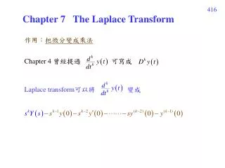
Chapter 2 Laplace Transform 2.1 Introduction • The Laplace transform method can be used for solving linear differential equations. • Laplace transforms can be used to convert many common functions, such as sinusoidal functions, damped sinusoidal functions, and exponential functions into algebraic functions of a complex variable s. • Operalions such as differentiation and integration can be replaced by algebraic operations in the complex plane.Thus, a linear differential equation can be transformed into an algebraic equation in a complex variable s.
ข้อดีของLaplace transform • It allows the use of graphical techniques for predicting the system performance without actually solving system differential equations. • When we solve the differential equation, both the transient component and steady state component of the solution can be obtained simultaneously.
Complex variables • Use notation s as a complex variable; that is, s = + jt where is the real part and is the imaginary part. 2.2 Review of complex variables and complex functions Complex function • A complex function F(s), a function of s, has a real part and an imaginary part or F(s) = Fx+ jFy where Fxand Fyare real quantities.
Points at which the function G(s) or its derivatives approach infinity are called poles. พิจารณาComplex function G(s) • If G(s) approaches infinity as s approaches -p and if the function G(s)(s + p)n, for n = 1, 2, 3, ... has a finite, nonzero value at s = - p, then s = -p is called a pole of order n. If n = 1, the pole is called a simple pole. If n = 2, 3, ... , the pole is called a second-order pole, a third order pole, and so on. • As an example, consider the following G(s):
Points at which the function G(s) equals zero are called zeros. • To illustrate, consider the complex function G(s) has zeros at s = -2, s = -10, simple poles at s = 0, s = -1, s = -5, and a double pole (multiple pole of order 2) at s = -15. Note that G(s) becomes zero at s = . Since for large values of s G(s) possesses a triple zero (multiple zero of order 3) at s =.
Euler’s Theorem. The power series expansions of cosand sinare, respectively, Euler’s Theorem; (2-1)
By using Euler's theorem, we can express sine and cosine in terms of an exponential function. • Noting thate-jis the complex conjugate of ejand that • we find, after adding and subtracting these two equations, that
Let us define f(t) = a function of time t such that f(t) = 0 for t < 0 s = a complex variable L = an operational symbol indicating that the quantity that it prefixes is to be transformed by the Laplace integral F(s) = Laplace transform of f(t) 2.3 Laplace Transformation Then the Laplace transform of f(t) is given by
The inverse Laplace transformation (2-4) • The time function f(t) is always assumed to be zero for negative time; that is, f(t) = 0, for t < 0
Laplace transform thus obtained is valid in the entire s plane except at the pole s = 0.
The step function whose height is unity is called unit-step function. • The unit-step function that occurs at t = tois frequently written as 1(t - to). • The step function of height A that occurs at t = 0 can then be written as f(t) = A1(t). • The Laplace transform of the unit-step function, which is defined by1(t) = 0, for t < 0 1(t) = 1, for t > 0 is 1/s,or • Physically, a step function occurring at t = 0 corresponds to a constant signal suddenly applied to the system at time t equals zero.
2.5 Inverse Laplace Transform • Important notes - The highest power of s in A(s) mustbe greater than the highest power of s in B(s). - If such is not the case, the numerator B(s) must be divided by the denominator A(s) in order to produce a polynomial in s plus a remainder