Download
1 / 17
170 likes | 288 Vues
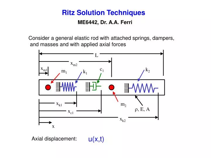
Ritz Solution Techniques. ME6442, Dr. A.A. Ferri. Consider a general elastic rod with attached springs, dampers, and masses and with applied axial forces. u(x,t). Axial displacement:. Kinetic energy of the elastic rod. could be r (x)A(x). Total kinetic energy.

E N D
Ritz Solution Techniques ME6442, Dr. A.A. Ferri Consider a general elastic rod with attached springs, dampers, and masses and with applied axial forces u(x,t) Axial displacement:
Kinetic energy of the elastic rod could be r(x)A(x) Total kinetic energy Potential energy of the elastic rod could be E(x)A(x) Total potential energy
Virtual Work of a single axial point force: Virtual work associated with a distributed force per unit length f(x,t) Total virtual work of applied forces
Rayleigh Dissipative Function External viscous damping Internal viscous damping isolated viscous dampers At this point, we have expressions for kinetic energy, potential energy, Rayleigh dissipation function, and virtual work. We are very close to being able to use the standard, discrete form of Lagrange’s equations, except for the integral terms. To handle this, we need some sort of discretization technique--- Ritz expansions
Expand displacement field as a finite summation of Ritz vectors (also called basis vectors) multiplied by time-varying generalized coordinates. This has the effect of turning an infinite-dimensional problem (governed by partial differential equations PDE’s) into a set of N ordinary differential equations (ODE’s). Substitute Ritz expansion into kinetic energy expression:
Collecting terms, we get where Similarly, inserting the Ritz expansion into the potential energy expression:
Collecting terms, we get where Similarly, inserting the Ritz expansion into the Rayleigh dissipation function: where
Substituting the Ritz expansion into the virtual work yields where Substitute T, V, D, and Qj into Lagrange’s equations Yields N coupled, second-order, ordinary differential equations
Problem 6.5 Non-uniform axial rod Ritz vectors expansion Need to choose y functions that satisfy the geometric boundary conditionsof the problem
choose Note that y(0) = y(L) = 0 Kinetic energy:
Mass terms Introduce variable
After applying Lagrange’s equations, get a system of linear equations Define
N = 4 mhat = 0.7500 -0.0901 -0.0000 -0.0072 -0.0901 0.7500 -0.0973 -0.0000 -0.0000 -0.0973 0.7500 -0.0993 -0.0072 -0.0000 -0.0993 0.7500 khat = 7.4022 -2.2222 -0.0000 -0.6044 -2.2222 29.6088 -6.2400 -0.0000 -0.0000 -6.2400 66.6198 -12.2449 -0.6044 -0.0000 -12.2449 118.4353 natfreqs = 3.1233 6.2746 9.4198 12.5790 times
PHI = 1.1612 0.0698 -0.0075 -0.0066 0.0718 1.1686 -0.0769 -0.0090 0.0076 0.0776 -1.1700 -0.0789 0.0064 0.0075 -0.0775 -1.1626 Now, need to convert eigenvectors PHI into continuous, eigenfunctions Define nth eigenfunction For example,
What if the rod was not tapered? mhat = 0.5000 -0.0000 0.0000 -0.0000 -0.0000 0.5000 0.0000 0.0000 0.0000 0.0000 0.5000 -0.0000 -0.0000 0.0000 -0.0000 0.5000 khat = 4.9348 -0.0000 -0.0000 -0.0000 -0.0000 19.7392 0.0000 0.0000 -0.0000 0.0000 44.4132 0.0000 -0.0000 0.0000 0.0000 78.9568 Note that the mass and stiffness matrices are now diagonal. This implies that the equations of motion are uncoupled. This happens because the Ritz vectors are the exact eigenfunctions for this problem.