Download
1 / 19
190 likes | 379 Vues
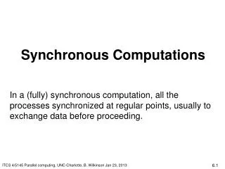
Synchronous Computations Chapter 6. Synchronous Computations. . In a (fully) synchronous application, all the processes synchronized at regular points MPI_Barrier () A basic mechanism for synchronizing processes

E N D
Synchronous Computations Chapter 6
Synchronous Computations . In a (fully) synchronous application, all the processes synchronized at regular points MPI_Barrier() A basic mechanism for synchronizing processes Called by each process in the group, blocking until all members of the group have reached the barriercall and only returning then
Barrier Implementation Centralized counter implementation (a linear barrier):
Fully Synchronized Computation Examples • Data Parallel Computations • Same operation performed on different data elements • simultaneously; i.e., in parallel. • Particularly convenient because: • Ease of programming (essentially only one program). • Scale easily to larger problem sizes. • Many numeric and some non-numeric problems can be cast in a data parallel form
Prefix Operations • Given a list of numbers, x0, …, xn-1, compute all the partial summations, i.e.: • x0x0+ x1x0 + x1 + x2x0 + x1 + x2 + x3 … • Any associative operation (e.g. ‘+’, ‘*’, Bitwise-AND etc.) can be used. • Practical applications in areas such as sorting, recurrence relations, and polynomial evaluation.
MIMD Powershift on a Hypercube Shift-by-2k(in Gray-Code Order) can be done in two routing steps on a hypercube Example: Shift-by 4 on a 16 PE hypercube 0 1 000 001 011 010 - 110 111 101 100 o 100 101 111 110 - 010 011 001 000 A B C D - E F G H o I J K L - M N O P wid: 000 001 011010 110 111 101 100 1) shift-by-2 in reverse order P O B A - D C F E o H G J I - L K N M 2) shift-by-2 again (in reverse order) M N O P - A B C D o E F G H - I J K L Tpar = 2 routing steps = O(1)
MIMD Powershift on a Hypercube Shift-by-2k(in Gray-Code Order) can be done in two routing steps on a hypercube Example: Shift-by 8 on a 16 PE hypercube 0 1 000 001 011 010 - 110 111 101 100 o 100 101 111 110 - 010 011 001 000 A B C D - E F G H o I J K L - M N O P wid: 00 0111 10 1) shift-by-4 in reverse order P O N M - D C B A o H G F E o L K J I 2) shift-by-4 again (in reverse order) I J K L - M N O P o A B C D - E F G H Tpar = 2 routing steps = O(1)
Solving a General System of Linear Equations where x0, x1, x2, … xn-1 are the unknowns • xiis expressed in terms of the other unknowns • This can be used as an iteration formula for each of the unknowns to obtain better approximations. By rearranging the ith equation:
Parallel Jacobi iterations P0 P1 Pn-1 Jacobi method will converge if diagonal value aii (i, 0 ≤ i< n) has an absolute value greater than the sum of the absolute values of the other aij’s on the same row. Then A matrix is called diagonally dominant: If P << n, how do you do the data & task partitioning?
Termination Compare values computed in one iteration to values obtained from the previous iteration. Terminate computation when all values are within given tolerance: or: In either case, you need a ‘global sum’ (MPI_Reduce) operation. Q: Do you need to execute it after each and every iteration ?
Parallel Code Process Pi could be of the form x[i] = b[i]; /*initialize unknown*/ for (iter = 0; iter < limit; iter++) { sum = -a[i][i] * x[i]; for (j = 0; j < n; j++) /* compute summation */ sum = sum + a[i][j] * x[j]; new_x[i] = (b[i] - sum) / a[i][i]; /* compute unknown */ All-to-All-Broadcast(&new_x[i]); /*bcast/rec values */ Global_barrier(); /* wait for all procs */ }
Other fully synchronous problems Cellular Automata • The problem space is divided into cells. • Each cell can be in one of a finite number of states. • Cells affected by their neighbors according to certain rules, and all cells are affected simultaneously in a “generation.” • Rules re-applied in subsequent generations so that cells evolve, or change state, from generation to generation. • Most famous cellular automata is the “Game of Life” devised by John Horton Conway, a Cambridge mathematician.
The Game of Life Board game - theoretically infinite 2-dimensional array of cells. Each cell can hold one “organism” and has eight neighboring cells. Initially, some cells occupied. The following rules were derived by Conway after a long period of experimentation: 1. Every organism with two or three neighboring organisms survives for the next generation. 2. Every organism with four or more neighbors dies from overpopulation. 3. Every organism with one neighbor or none dies from isolation. 4. Each empty cell adjacent to exactly three occupied neighbors will give birth to an organism.
Simple Fun Examples of Cellular Automata “Sharks and Fishes” An ocean could be modeled as a 3-dimensional array of cells. Each cell can hold one fish or one shark (but not both). Fish Might move around according to these rules: If there is one empty adjacent cell, the fish moves to this cell. If there is more than one empty adjacent cell, the fish moves to one cell chosen at random. If there are no empty adjacent cells, the fish stays where it is. If the fish moves and has reached its breeding age, it gives birth to a baby fish, which is left in the vacating cell. Fish die after x generations.
Sharks Might be governed by the following rules: If one adjacent cell is occupied by a fish, the shark moves to this cell and eats the fish. If more than one adjacent cell is occupied by a fish, the shark chooses one fish at random, moves to the cell occupied by the fish, and eats the fish. If no fish are in adjacent cells, the shark chooses an unoccupied adjacent cell to move to in a similar manner as fish move. If the shark moves and has reached its breeding age, it gives birth to a baby shark, which is left in the vacating cell. If a shark has not eaten for y generations, it dies.