1 / 0

Ch. 5: Supply

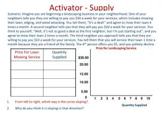
Ch. 5: Supply. Sec. 1: What Is Supply?. Supply- anyone who provides goods & services is a producer manufacturers, farmers, airlines, utility comp., pet sitter Key words – if prices to low – some not willing to take on expense of growing and transport

finley
Télécharger la présentation

Ch. 5: Supply

An Image/Link below is provided (as is) to download presentation Download Policy: Content on the Website is provided to you AS IS for your information and personal use and may not be sold / licensed / shared on other websites without getting consent from its author. Content is provided to you AS IS for your information and personal use only. Download presentation by click this link. While downloading, if for some reason you are not able to download a presentation, the publisher may have deleted the file from their server. During download, if you can't get a presentation, the file might be deleted by the publisher.

E N D

Presentation Transcript


  1. Ch. 5: Supply

  2. Sec. 1: What Is Supply? Supply- anyone who provides goods & services is a producer manufacturers, farmers, airlines, utility comp., pet sitter Key words – if prices to low – some not willing to take on expense of growing and transport bad weather – not able to supply a farmers market
  3. The Law of Supply The law of supply – producers want to earn a profit when prices rises – when price falls –
  4. Example: Price and Supply Smith family – sell at Montclair farmers market – lots of f & v, special – tomato how to price the tomatoes @ $1 per lbs. – supply 24 lbs to market @ $2 per lbs – supply 50 lbs to market @ $.50 pr lbs – supply 10 lbs or even none
  5. Supply Schedule Supply schedule – shows law of supply in table form Market supply schedule –
  6. Example: Individual Supply Schedule 2 column table similar to a demand schedule left hand column – various prices of a good or service right hand column – quantity supplied at each price Figure 5.2 – Smith’s supply schedule
  7. Example: Market Supply Schedule Several stands sell tomatoes at the market want to know the quantity of tomatoes available for sale at different prices for the entire farmers market – need a market supply schedule shows quantity supplied by all the producers who are willing and able
  8. Example: Market Supply Schedule Figure 5.3 – similar to supply schedule only quantities are larger market quantity supplied depends on price market research can be used to create a market supply schedule Producers use research done by govt. or trade organizations
  9. Supply Curves Supply curve – Market supply curve – shows how much of a good or service all of the producers in a market are willing or able to offer for sale at each price
  10. Example: Individual Supply Curve Figure 5.4 – Smith’s supply schedule when price increases – when price decreases – created using the assumption that all other economic factors except price remain the same
  11. Example: Market Supply Curve Figure 5.5 Shows the quantity of tomatoes that all the producers (the market as a whole) are willing and able to offer for sale at each price differs in scope, but is made the same way direct relationship between price and quantity supplied if price increases among all suppliers then quantity supplied increases if price decreases, then quantity supplied decreases constructed on assumption that all other economic factors remain the same Supply curves for all producers follow the law of supply does not matter what is produced why spend more when prices are higher higher prices signal potential for higher profits
  12. Market Supply Schedule
  13. Sec. 2: What Are the Costs of Production?
  14. Labor Affects Production Marginal product – Janine’s jean factory – 3 workers produce 12 pairs each day increase the # of workers and output increases adding a 5th worker allows for specialization Specialization –
  15. Example: Marginal Product Schedule Shows relationship between labor and marginal product Figure 5.7 1 or 2 workers produce very little, but it is bigger with each one between 3 & 6 workers allows for specialization, higher production Increasing returns – Diminishing returns – workers 7,8,9,10 work overlaps with 1st 6 workers with worker 11, total output decreases employees crowded, operations disorganized this is rare, but it can happen
  16. Production Costs Goal is to make a profit – Fixed costs – are expenses that the owners of a business must incur whether they produce nothing, a little , or a lot Variable costs – Total cost – adding fixed and variable costs together Marginal costs –
  17. Example: Fixed and Variable Costs Janine fixed costs – the same whether producing or not salaries of managers who run the company, but not involved directly in production Variable costs – increase production and variable cost go up decrease production (cut back hours, vacation for a week), variable cost decrease To determine total cost of a pair of jeans –
  18. Example: Production Costs Schedule Figure 5.8 – see costs and how they change as quantity of jeans produced changes # of workers added is a major factor fixed costs stay the same no matter what the total product amounts to Marginal cost is determined by marginal cost decline b/c of specialization but then increases b/c of diminishing returns
  19. Production Costs Schedule
  20. Earning the Highest Profit Marginal revenue – it is the price Total revenue – Formula – Total Revenue= P x Q P= price of the product Q= quantity purchased at that price
  21. Example: Production Costs and Revenue Schedules Janine & figure 5.9 finds total revenue by multiplying marginal revenue by total product determine profit by subtracting total costs from total revenue wants to know how many workers to hire and how many pairs of jeans to make to get most profit need to perform a marginal analysis – a comparison of added costs and benefits Examine figure 5.9 with 1 worker – does not make a profit at 2 workers – earns a profit and passes break-even point – total costs and total revenue are exactly the same profits continue to rise up to and including the 9th worker Profit-maximizing output – reached a level where it has achieved the highest level of profit marginal revenue and marginal cost are equal then profits begin to decline at 10th worker – increase in marginal cost is greater than increase in marginal revenue
  22. Production Costs & Revenue Schedule
  23. Sec. 3 What Factors Affect Supply?

  24. Changes in Quantity Supplied Early curves created using the assumption that all other economic factors except price remain the same The only thing influence how much producers will offer for sale is price Supply curve shows that pattern different points on supply curve show change in quantity supplied Change in quantity supplied –
  25. Example: Changes Along a Supply Curve Each new point shows a change in quantity supplied a change in quantity supplied - change is shown by the direction of movement along the curve to the right – to the left – Figure 5.10 shows individual information market supply curve show similar info for an entire market they just have large quantities supplied
  26. Changes in Supply Change in supply – production costs increase – production costs decrease – 6 factors can cause a change in supply: input costs, labor productivity, technology, govt. action, producer expectations, number of producers
  27. Decrease Increase
  28. Factor 1: Input Costs Input costs – Anna and nutrition bars made with peanuts price of peanuts increases – cannot afford to produce as many bars supply curve shifts to the left - & vice versa
  29. Factor 2: Labor Productivity Labor productivity – increased productivity decreases the costs of production – increases supply specialized division of labor allows for making more goods at a lower cost better trained and more skilled workers can usually produce more goods in less time and lower costs then less educated and less skilled
  30. Factor 3: Technology Technology – technology used to make goods more efficiently increased automation leads to increased supplies allows workers to be more productive and helps business to increase the supply of their services
  31. Factor 4: Government Action Excise tax – often placed on alcohol & tobacco (govt. interested in discouraging use) increases producer cost, decreases supply Taxes tend to decrease supply, subsidy do the opposite Regulation – can affect supply banning a pesticide can decrease the supply of the crops that depend on it worker safety can decrease supply by increasing production costs or increase supply by reducing labor lost to on the job injuries
  32. Factor 5: Producer Expectations If producers expect price of their product to rise or fall, producers each react differently if farmer expects corn prices to rise –
  33. Factor 6: Number of Producer When one company develops a new idea, other producers will enter the market and increase the supply of the good or service supply curve shifts to the right – figure 5.13 increase in # of producers means increased competition may drive less efficient producers out of the market – decreasing supply
  34. Figure 5.13 – ice cream stores one starts – is a success – 6 months later – 3 more stores supply of ice cream cones increased all price levels within 1 yr., one forced out of the market
  35. Economic Pacesetter: Robert Johnson: Supplying African –American Entertainment Media entrepreneur – b. April 8, 1946 1970s – Washington lobbyist for National Cable Television Association recognized void of African American TV market Conceived idea for Black Entertainment Television (BET) took $15,000 loan and secured a $500,000 investor picked up a space on cable TV started on Jan. 8, 1980 started with 2 hours of programming a week
  36. Today – 5 separate channels – operators in US, Canada, Caribbean at 1st – shows similar to MTV later – more diverse programming BET.com - #1 internet portal for African-Americans 2001 – sold BET to Viacom International for $3 Billion became 1st black billionaire continued to run company for 5 yrs. companies began to copy Johnson’s ideas for programming for the African-American community
  37. Sec. 4: What Is Elasticity of Supply?
  38. Elasticity of Supply Toyota introduces hybrid Prius in 2000 instant success – not able to increase supply at same pace that consumer demand and prices rose 5 yrs. Later – not meet growing demand inability to meet increased demand suggests the supply is inelastic Elasticity of supply – if a change is price leads to a relatively larger change in quantity supplied - a 10% increase in price causes a greater than 10% increase in quantity supplied if a change in price leads to a relatively smaller change in quantity supplied – if the price and quantity supplied change by the exact same % -
  39. Example: Elastic Supply Figure 5.15 shows quantity supplied of new leather boots – gained popularity, shortage developed is elastic price was raised – and quantity supplied kept up producer able to keep up because raw materials are inexpensive & easy to get manufacturing process is also fairly uncomplicated and easy to increase
  40. Example: Inelastic Supply Figure 5.16 – olive oil supply of olive oil is inelastic price rose by a factor of 4, supply could not keep pace oil comes from previous seasons olives
  41. What Affects Elasticity of Supply? Ease of changing production to respond to price change is the main factor in determining elasticity of supply supply is more elastic over time – a year or several years Industries that are able to respond quickly to changes in price by either increasing or decreasing production are those that don’t require a lot of capital, skilled labor or difficult to obtain resources dog-walkers a business that sells small crafts industries that would have trouble – auto & oil refiners takes time to respond to price changes
More Related