Download
1 / 18
290 likes | 632 Vues
The Coupled Magnetosphere-Ionosphere-Thermosphere Model, v. 2.0: Ionospheric Electrodynamics. Stan Solomon, Alan Burns, Jiuhou Lei, Astrid Maute, Art Richmond, Wenbin Wang, Mike Wiltberger, and Janet Zeng High Altitude Observatory National Center for Atmospheric Research.

E N D
The Coupled Magnetosphere-Ionosphere-Thermosphere Model, v. 2.0:Ionospheric Electrodynamics Stan Solomon, Alan Burns, Jiuhou Lei, Astrid Maute, Art Richmond, Wenbin Wang, Mike Wiltberger, and Janet Zeng High Altitude Observatory National Center for Atmospheric Research CISM Advisory Council Meeting • Boston University • 12 March 2007
CMIT v. 1.1 LFM Jll, np,Tp E Magnetosphere - Ionosphere Coupler (H+P)=Jll-Jw Particle precipitation: Fe, E0 Conductivities: p, h, Winds: Jw Electric Potential: tot TING CMIT 1.0 (no Jw feedback) delivered to CCMC
CMIT v. 2.0 LFM Jll, np,Tp E Magnetosphere - Ionosphere Coupler (H+P)=Jll-Jw Particle precipitation: Fe, E0 Conductivities: p, h, Winds: Jw Electric Potential: tot TIE-GCM GSWM Neutral wind feedback standard Intercomm coupling standard
How is TIE-GCM different from TING? • Physical Differences: • TIE-GCM calculates the low-latitude electric field using the modeled neutral winds • Apex magnetic coordinate system employed (based on IGRF) • (TIGCM and TING used dipole magnetic field and empirical electric field) • TIE-GCM can use a lower boundary tidal specification from the GSWM • (Global Scale Wave Model) • TIE-GCM has a new solar ionization method and improved photochemistry • …and can be driven using measured solar EUV irradiance • TIE-GCM has improved validation with neutral density and ionospheric data • …a work in progress • Numerical Differences: • TING is a serial code • TIE-GCM is a MPI code with 2-D decomposition in geographic latitude, longitude • …but, the dynamo potential solver is in mag. coordinates, and still serial • Input/output files standardized in netCDF, graphics/analysis packages, etc. • High-resolution (2.5° x 2.5° x H/4) version in the works
Low-Latitude Dynamo Creates the Appleton Anomaly a.k.a., equatorial ionization anomaly, intertropical arcs, tropical nightglow, etc.
Calculation of the Global Ionospheric Electric Potential • Basic assumptions: • Steady-state, electrostatic electric field • No electric field along magnetic field lines • Current density in divergence-free current density magnetospheric term wind-driven “dynamo” terms field-aligned current This results in the potential equation, which is solved for high latitudes in the M-I coupling module: wind-driven current field-line integrals conductance field-line integral • We would like to solve this equation at all latitudes, however, there are two problems: • The dynamo solver is hemispherically symmetric, but Jmr is not • We don’t yet have a full description of the region-2 current system
Calculation of the Global Ionospheric Electric Potential In CMIT 2.0, these difficulties are circumvented using the same approach used to combine an empirical or assimilated high-latitude potential with the TIE-GCM low-latitude dynamo: global potential mean high-latitude potential p is a cross-over parameter: p=1 below magnetic latitude 60° and p=0 above 75°. Using this formulation, we are getting a “partially shielded” low-latitude ionosphere that allows some penetration electric fields, but neglects the time-dependent aspect because there is no explicit region-2 current system. When coupled with the LFM, we get a little more shielding, since the LFM does contain weak region-2 currents.
Comparison with Ionospheric Measurements by COSMIC Jiuhou Lei et al., “Comparison of COSMIC ionospheric measurements with ground-based observations and model predictions: preliminary results,” J. Geophys. Res., in press, 2007.
Equatorial Vertical Drift — Comparison with Jicamarca Data Vertical Drift (m/s) Vertical Drift (m/s)
Next Steps in the Development of a Global Potential Solver Instead of using an applied potential at high latitudes and the cross-over function, apply magnetospheric field-aligned currents directly to the solver: Then, solve the three regions separately, and iterate between solutions to obtain convergence at the two interfaces: global potential low latitudes high latitudes 90 high lat. boundary NH NH 54 interface low lat. boundary NH = + equator mag. latitude SH symmetric low lat. boundary -54 interface SH SH -90 -180 mag. longitude 180
Next Steps in the Development of a Global Potential Solver • We have implemented and tested this iterative dynamo solver, but only for individual time-steps — it is not yet part of CMIT. • For this to work effectively, we need: • • Improved description of time-dependent region-2 current system • Complete integration of RCM into CMIT • • Improved efficiency of dynamo routine • Parallelize field-line integral calculations • Parallelize elliptical solver routine