Download
1 / 13
130 likes | 289 Vues
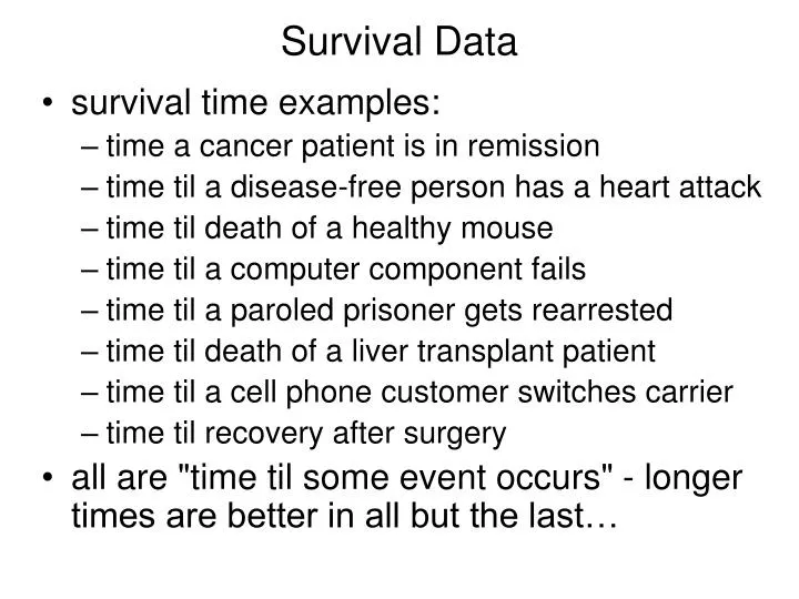
Survival Data. survival time examples: time a cancer patient is in remission time til a disease-free person has a heart attack time til death of a healthy mouse time til a computer component fails time til a paroled prisoner gets rearrested time til death of a liver transplant patient

E N D
Survival Data • survival time examples: • time a cancer patient is in remission • time til a disease-free person has a heart attack • time til death of a healthy mouse • time til a computer component fails • time til a paroled prisoner gets rearrested • time til death of a liver transplant patient • time til a cell phone customer switches carrier • time til recovery after surgery • all are "time til some event occurs" - longer times are better in all but the last…
Three goals of survival analysis • estimate the survival function • compare survival functions (e.g., across levels of a categorical variable - treatment vs. placebo) • understand the relationship of the survival function to explanatory variables ( e.g., is survival time different for various values of an explanatory variable?)
The survival function S(y)=P(Y>y) can be estimated by the empirical survival function, which essentially gets the relative frequency of the number of Y’s > y… • Look at Definition 1.3 on p.5: Y1, … ,Yn are i.i.d. (independent and identically distributed) survival variables. Then Sn(y) =empirical survival function at y = (# of the Y’s > y)/n = estimate of S(y). • Note that where I is the indicator function…
Review of Bernoulli & Binomial RVs: • Show that the expected value of a Bernoulli rv Z with parameter p (i.e., P(Z=1)=p) is p and that the variance of Z is p(1-p) • Then knowing that the sum of n iid (independent and identically distributed) Bernoullis is a Binomial rv with parameters n and p, show on the next slide that the empirical survivor function Sn(y) is an unbiased estimator of S(y)
Note that and as such nSn has B(n,p) where p=P(Y>y)=S(y). • Also note that for a fixed y* so Sn is unbiased as an estimator of S • What is the Var(Sn)? (see 1.6 and on p.6 where the confidence interval is computed…) • Try this for Example 1.3, p.6
Example 1.4 on page 8 shows that it is sometimes difficult to compare survival curves since they can cross each other… (what makes one survival curve “better” than another?) • One way of comparing two survival curves is by comparing their MTTF (mean time til failure) values. Let’s try to use R to draw the two curves given in Ex. 1.4: S1(y)=exp(-y/2) and S2(y)=exp(-y2/4)… see the handout R#1.
Note that the MTTF of a survival rv Y is just its expected value E(Y). We can also show (Theorem 1.2) that (Math & Stat majors: Show this is true using integration by parts and l’Hospital’s rule…!) • So suppose we have an exponential survival function: (btw, can you show this satisfies the properties of a survival function?)
Then the MTTF for this variable is - show this… • And for any two such survival functions, S1(y)=exp(-y/ and S2(y)=exp(-y/ one is “better” than the other if the corresponding beta is “better”… • HW: Use R to plot on the same axes at least two such survival functions with different values of beta and show this result.
The hazard function • The hazard function gives the so-called “instantaneous” risk of death (or failure) at time t. Recall that for continuous rvs, the probability of occurrence at time t is 0 for all t. So we think about the probability in a “small” interval around t, given that we’ve survived to t, and then let the small interval go to zero (in the limit). The result is given on page 9 as the hazard rate or hazard function…
Definition of hazard function: • notes • the hazard function is conditional on the individual having already survived to time y • the numerator is a non-decreasing function of y (it is more likely that Y will occur in a longer interval) so we divide by the length of the interval to compensate • we take the limit as the length of the interval gets smaller to get the risk at exactly y - “instantaneous risk”
we can show (see p.9) that the hazard function is equal to • use f(y)=-d/dy(S(y)) and the above to show that • so all three of f, h, and S are representations that can be found from the others and are used in various situations…
more notes on the hazard function: • hazard is in the form of a rate - hazard is not a probability because it can be >1, but the hazard must be > 0; so the graph of h(y) does not have to look at all like that of a survivor function • in order to understand the hazard function, it must be estimated. • think of the hazard h(y) as the instantaneous risk the event will occur per unit time, given that the event has not occurred up to time y. • note that for given y, a larger S(y) corresponds to a smaller h(y) and vice versa…
life expectancy at age t: • if Y=survival time and we know that Y>t, then Y-t=residual lifetime at age t and the mean residual lifetime at age t is the conditional expectation E(Y-t|Y>t) = r(t) • it can be shown that • note that when t=0, r(0)=MTTF • we define the mean life expectancy at age t as E(Y|Y>t) = t +r(t) • go over Example 1.6 on page 11…