Download

1 / 65
650 likes | 669 Vues
PHASOR FUNDAMENTALS. HANDS-ON RELAY SCHOOL 2019 Steve Laslo System Protection and Control Specialist Bonneville Power Administration. Presentation Information. This presentation is a revision to Phasor Diagrams , presented at the Hands-On Relay School for many years by Ron Alexander.

E N D
PHASOR FUNDAMENTALS HANDS-ON RELAY SCHOOL 2019 Steve Laslo System Protection and Control Specialist Bonneville Power Administration
Presentation Information • This presentation is a revision to Phasor Diagrams, presented at the Hands-On Relay School for many years by Ron Alexander. • Much of the content in this presentation is based on J. Lewis Blackburn’s fantastic reference: Protective Relaying Principles and Applications (multiple editions). • Our Primary Objective for this presentation is to enhance attendee knowledge by: • Reviewing Phasor fundamentals • Examining In-Service/Load checks • Our Secondary Objective (time permitting) will add: • Reviewing Fault Phasors • Using phasors to determine phase shift across three-phase transformer banks
Phasors – Why? • Tool for understanding the power system during load and fault conditions. • Assists a person in understanding principles of relay operation for testing and analysis of relay operations. • Allows technicians to simulate faults that can be used to test relays. • Common language of power protection engineers and technicians. • Provides both mathematical and graphical view of System conditions.
Phasor Definitions • A line used to represent a complex electrical quantity as a vector. (Google) • A rotating vector representing a quantity, such as an alternating current or voltage, that varies sinusoidally. (Collins Dictionary) • A vector that represents a sinusoidally varying quantity, as a current or voltage, by means of a line rotating about a point in a plane, the magnitude of the quantity being proportional to the length of the line and the phase of the quantity being equal to the angle between the line and a reference line. (Dictionary.com)
Phasor Rotation • Here we can see a plot of an electrical quantity and its phasor representation. • Note the phasor has a constant (usually RMS) magnitude that rotates while the actual electrical quantity varies sinusoidally over time.
Multiple Phasors • Here we can see two phasors of the same frequency rotating. • Note that their phase relationship to each other is constant – in this case, the blue phasor leads the red phasor by some constant angle that does not change.
PLOTTING PHASORS * V P I CARTESIAN COORDINATE SYSTEM
Phasor Representation • Consider an example phasor ‘c’ having a magnitude of 120VRMS and a phase angle of 30 degrees: • Rectangular Form: c = x + jy • c = 104 + j60 V • Polar Form: c = |c|θ • c = 12030° V • Complex Form: c = |c|(cosθ + jsinθ) • c = 120(cos(30) + jsin(30)) V • Exponential Form: c = |c|ejθ • c = 120ej30 V
Phasor Conversion • Rectangular <> Polar Conversion: • Rectangular Form: c = x + jy • c = 104 + j60 • Polar Form: c = cθ • c = 12030° • Trig Functions (right triangles only): • Sin(θ) = opposite / hypotenuse • Cos(θ) = adjacent / hypotenuse • Tan(θ) = opposite / adjacent • Pythagorean Theorem • c2 = a2 + b2
Phasor Conversion • Rectangular to Polar Conversion: • Rectangular Form: c = x + jy • c = 104 + j60 • c2 = a2 + b2 • c2 = 1042 + 602 >> c = 120 • Tan (θ) = opposite / adjacent • Tan (θ) = 60 / 104 >> θ = 30° • Converted: c = 12030°
Phasor Conversion • Polar to Rectangular Conversion: • Polar Form: c = |c|θ • c = 12030° • Sin(θ) = o/h • o = h* Sin(θ) • o = 120 * Sin(30) = 60 • Cos(θ) = a/h • a = h * Cos(θ) • a = 120 * Cos(30) = 104 • Converted: c = 104 + j60
Operators • Two ‘Operators’ related to phasors are commonly used in the Power world: ‘j’ and ‘a’ • Mathematically ‘j’ is an imaginary number representing the imaginary (reactive) portion of a phasor: j = -1 • Graphically, it is a ‘rotator’ constant with an angle of 90° • It can also be viewed as a ‘unit phasor’ always having a value of 190° • The ‘a’ Operator, commonly used when working with Symmetrical Components. • Graphically it is a ‘rotator’ constant with an angle of 120° • It is also a ‘unit phasor’ with a value of 1120°
Combining Phasors • Two common operations are performed with phasors: • Adding / Subtracting • Multiplying / Dividing • It’s generally easier to add/subtract in rectangular form and easier to multiply/divide in polar form. • When adding/subtracting in rectangular form, add/subtract the real and reactive components (respectively): • Example: (2+j3) + (3+j4) = (5+j7) • When multiplying/dividing in polar form, multiply/divide the magnitude, and add/subtract the angle: • Example: (1030°) * (545°) = 5075°)
Adding Phasors Graphically • You can also add vectors graphically by connecting them head to tail. • The resultant is the phasor originating at the origin of the first arrow and ending at the head of the last arrow. • Here, if we have the following: • Va = 1200°V • Vb = 120-120°V • Vc = 120120°V • Va + Vb + Vc = 0
Adding Phasors Graphically • In this example, the VAB voltage is VA-VB. We subtract VB by reversing the VB phasor and adding it to VA. • VAB = VA-VB = VA+(-VB)
Sinusoidal Waveforms • Note that adding or subtracting sinusoidal waveforms simply produces a resultant sinusoidal waveform of the same frequency.
Phasors – Conjugation • Most commonly used in power calculation: P=EI where the conjugate of I is sometimes used and shown as: P=EI* • Conjugates: • c = x - jy • c = c- • c = |c|(cos - jsin) • c = |c|e-j
Phasors – Conjugation • Calculating: P = E * I we get: • P = 1200°V * 0.42-45°A = 50.9-45°VA • Placing this phasor on one of our previous Power Flow diagrams gives →→→ • But Blackburn and many others use +Q in the 1st Quadrant. • If we calculate P using the conjugate of the current: P = E * I* • P = 1200°V * 0.42 +45°A = 50.9+45°VA • This places P in the 1st Quadrant.
Phasors – Conjugation • It’s extremely important to remember that phasor diagrams are descriptors of circuit information. How they are placed on a diagram does not change the electrical qualities of a circuit.
Phase Sequence • Phase Sequence is the order in which phasors pass a reference point. • In Symmetrical Components, you will hear the terms: positive sequence, negative sequence, and zero sequence. • Positive Sequence = ABC • Negative Sequence = ACB. • Zero sequence is all 3 phases rotating together at the same angle.
Resistor AC Response Phasor Diagram
Inductor AC Response Phasor Diagram
Capacitor AC Response Phasor Diagram
Phasor Nomenclature • Phasor diagrams can be drawn ‘open’ or ‘closed’.
Polarity • Current into the primary polarity and out of the secondary polarity are (essentially) in-phase. • Voltage drop from polarity to non-polarity on both windings are (essentially) in-phase.
Polarity and Phasors • When dealing with Phasors, we make assumptions about current and voltage polarity on our circuit diagram so polarity is also extremely important. • Consider the following circuit: we’ll do ‘in-service’ checks of the relays in the bottom current circuit. Chemawa Substation
Phasors in Practice • Here we’ve zoomed in on the current circuit we are interested in: • We’ll assume for convenience that the normal load flow for this circuit is from the Main Bus out into the line – the ‘up’ direction on this print.
Phasors in Practice • Now we’ll plan on where we will take secondary current readings. The test switches are made for this so we’ll use terminals 11/12, 15/16, and 19/20 on test switch 3L.
Phasors in Practice • We’ll also plan on checking the voltages to the relays for proper magnitude and polarity. • We’ll use the same 3L test switch, terminals 1-8.
Phasors in Practice • Which of the following phasor diagrams is correct for the circuit we are doing in-service on? • It is indeterminate / uncertain; both could be correct, or wrong… • Why? • We haven’t completed our circuit diagram (which we know should accompany our phasor diagram).
Phasors in Practice • Since we already assumed a load flow direction, now we just need to show on our circuit diagram our assumed polarity at our measurement point. • This determines how we ‘jack in’ to the current circuit using a phase-angle meter. In this diagram we will insert test equipment with assumed current ‘in’ on terminals 11, 15, and 19. IC IB Assumed Direction of Load Flow IA
Phasors in Practice • Let’s show/document our measurement points for the voltages too. • VAN = (3L) 1-7, VBN = (3L) 3-7, VCN = (3L) 5-7 VA VB VC VN
In-Service Sheet • Here is a in-service sheet based on our work and our measurements based on our circuit diagram. • What does it tell us? • It tells us our ‘assumed’ current direction was correct, and load is flowing from Chemawa to Santiam. It also tells us the load at Santiam is moderately Inductive. IC VCN VAN IB IA VBN 173 100
Phasors in Practice • Revisiting this slide, it appears Phasor Diagram #1 is correct – at least when it is paired with the circuit diagrams we’ve previously looked at. • But is Phasor Diagram #2 right or wrong? • Let’s consider that a 2nd Relay Technician took the phasor readings for diagram #2 and let’s consider that they used the following circuit diagrams.
Phasors in Practice • For Relay Technician #2 they assumed the direction of load flow was from Santiam to Chemawa – reverse to Technician #1. • Based on assumed current direction, Tech #2 ‘jacked in’ to the current circuit using a phase-angle meter with assumed current ‘in’ on terminals 12, 16, and 20. IC IB Assumed Direction of Load Flow IA
Phasors in Practice • Tech #2 used the same ‘across’ process for the voltages. • VAN = (3L) 1-7, VBN = (3L) 3-7, VCN = (3L) 5-7 VA VB VC VN
In-Service Sheet • Here is the in-service sheet for Tech #2. • What does it tell us? • It tells us our ‘assumed’ current direction was incorrect, and load is actually flowing from Chemawa to Santiam. It also tells us the load at Santiam is moderately Inductive. VCN IB VAN IA IC VBN 173 100
Phasors in Practice • Now we can see why the circuit diagram is vital in making a determination of whether phasors are correct… or not… • In this case, interpretation of the phasors proved both to be correct, when each is properly tied to its circuit diagram. • Phasors without an associated circuit diagram are essentially unprovable and of questionable value…
Phasor Fundamentals Review • Important Phasor fundamentals: • Phasor Representation • Phasor Nomenclature • Combining Phasors • Circuit Diagrams • Phase Rotation and Phase Sequence • Polarity • As Blackburn notes in his book: • Phasor fundamentals are essential aids in selection, connection, operation, performance, and testing of protection for power systems.
Fault Phasors • These fault types are (relatively) easy to understand; only one requires some consideration (Phase-to-Phase Fault) but even it is not hard once you consider some fault Fundamentals.
Fault Phasors • Transmission line faults are almost always inductive; let’s examine why: • Transmission line impedance is based on the length of line, the type of conductor, and the type and spacing of the structures the line is installed on. • When the line is loaded with normal shunt loads, the transmission line impedance is (for the most part) negligible and the loading and phase angle is determined by the load impedance; thus the load angles can be inductive/resistive/capacitive. • When a line faults, the load impedance is bypassed (shunted) and the fault current is limited by the source voltage and the impedance of the transmission line itself.
Fault Phasors • It’s important to note that given a uniform transmission line the fault angle will not vary for a fault anywhere on the transmission line.
Fault Phasors • Let’s look at some standard fault phasors. • To begin with, we’ll examine an ideal unfaulted system: • We’ll use VAN as our reference.
1LG Fault – AG • Assume a fault angle of 70° • Assume 50% voltage collapse • Key points: • VAN is reduced by 50% • IA increases and lags the Fault Voltage by the line angle, 70°
2LG Fault - BCG • Assume a fault angle of 70° • Assume 50% voltage collapse • Key points: • VBN and VCN are reduced by 50% • IB and IC increase and lags their Fault Voltage by the line angle, 70°
3LG Fault - ABCG • Assume a fault angle of 70° • Assume 50% voltage collapse • Key points: • All voltages are reduced by 50% • All currents increase and lag their Fault Voltage by the line angle, 70°