Download

1 / 13
350 likes | 955 Vues
~ Numerical Differentiation and Integration ~ Newton-Cotes Integration Formulas Chapter 21. Differentiation. and Integration. Calculus is the mathematics of change. Since engineers continuously deal with systems and processes that change, calculus is an essential tool of engineering.

E N D
~ Numerical Differentiation and Integration ~Newton-Cotes Integration FormulasChapter 21
Differentiation and Integration • Calculus is the mathematics of change. Since engineers continuously deal with systems and processes that change, calculus is an essential tool of engineering. • Standing at the heart of calculus are the concepts of:
Newton-Cotes Integration Formulas • Based on the strategy of replacing a complicated function or tabulated data with an approximating function that is easy to integrate: Zero order approximation First-order Second-order
The Trapezoidal Rule • Use a first order polynomial in approximating the function f(x) : • The area under this first order polynomial is an estimate of the integral of f(x) between a and b: Trapezoidal rule Error: where x lies somewhere in the interval from a to b
Example 21.1Single Application of the Trapezoidal Rulef(x) = 0.2 +25x – 200x2 + 675x3 – 900x4 + 400x5Integrate f(x) from a=0 to b=0.8 Solution:f(a)=f(0) = 0.2 and f(b)=f(0.8) = 0.232
The Multiple-Application Trapezoidal Rule • The accuracy can be improved by dividing the interval from a to b into a number of segments and applying the method to each segment. • The areas of individual segments are added to yield the integral for the entire interval. Using the trapezoidal rule, we get:
The Error Estimate for The Multiple-Application Trapezoidal Rule • Error estimate for one segment is given as: • An error for multiple-application trapezoidal rule can be obtained by summing the individual errors for each segment: Thus, if the number of segments is doubled, the truncation error will be quartered.
Simpson’s Rules • More accurate estimate of an integral is obtained if a high-order polynomial is used to connect the points. These formulas are called Simpson’s rules. Simpson’s 1/3 Rule: resultswhen a 2nd order Lagrange interpolating polynomial is used for f(x) a=x0x1 b=x2
The Multiple-Application Simpson’s 1/3 Rule • Just as the trapezoidal rule, Simpson’s rule can be improved by dividing the integration interval into a number of segments of equal width. • However, it is limited to cases where values are equispaced, there are an even number of segments and odd number of points.
Simpson’s 3/8 Rule Fit a 3rd order Lagrange interpolating polynomial to four points and integrate Simpson’s 1/3 and 3/8 rules can be applied in tandem to handle multiple applications with odd number of intervals
Newton-Cotes Closed Integration Formulas Same order, but Simpson’s 3/8 is more accurate In engineering practice, higher order (greater than 4-point) formulas are rarely used
Integration with Unequal Segments Using Trapezoidal Rule Example 21.7 which represents a relative error of e = 2.8% Data for f(x)= 0.2+25x-200x2+675x3-900x4+400x5
Compute Integrals Using MATLAB First, create a filecalledfx.mwhichcontains f(x): function y = fx(x) y = 0.2+25*x-200*x.^2+675*x.^3-900*x.^4+400*x.^5 ; Then, execute in thecommandwindow: >> Q=integral('fx', 0, 0.8) % true integral Q =1.6405 true value >> x=[0 .12 .22 .32 .36 .4 .44 .54 .64 .7 .8] >> y = fx(x) y = 0.200 1.309 1.305 1.743 2.074 2.456 2.843 3.507 3.181 2.363 0.232 >> I = trapz(x,y) % ortrapz(x, fx(x)) Integral =1.5948 Demo: (how I changeswrt n) + (0thorderapprox. Withlarge n).