Data Assimilation Workshop Notes

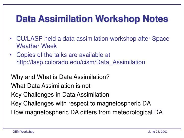
1. Why and What is Data Assimilation? What Data Assimilation is not Key Challenges in Data Assimilation Key Challenges with respect to magnetospheric DA How magnetospheric DA differs from meteorological DA Data Assimilation Workshop Notes • CU/LASP held a data assimilation workshop after Space Weather Week • Copies of the talks are available at http://lasp.colorado.edu/cism/Data_Assimilation

2. Purpose of data assimilation is to combine measurements and models to produce best estimate of current and future conditions. Kalman filter often used as a method for data assimilation. It became popular because it is a recursive solution to the optimal estimator problem. (Only last time step of information needs to be stored.) Full implementation of Kalman filter is usually not possible. There is a growing field in the study alternatives. Lessons LearnedWhy and What is DA? • AD ≠ DA (The Assimilation of Data is not necessarily Data Assimilation) • Data assimilation does not require a physics-based model.

3. Model Types Vector X contains all quantities on the grid, S is the external driver, M propagates the state forward • Linear: • Nonlinear: • Physical:

4. Challenges in DA • Analyzed field does not match a realizable model state • Non-uniform and sparse measurements • Observed variables do not match variables predicted by the model • Observing systems are diverse and subject to error, sometimes poorly known

5. Very sparse measurements Diverse set of both forward and inverse models that are highly specialized and/or are expert in different areas. Challenges For Magnetospheric DA • How to combine forward models (MHD, particle pushing) with inverse models (empirical, stochastic). • How to integrate data with these models

6. Meteorology Four- Dimensional Data Assimilation Combine Satellite, Aircraft, & Drift Buoys Continued Improvements Graphical to Mathematical Statistical Estimation & Prediction Physical Modeling 1940 1950 1960 1970 1980 1990 2000 2010 Physical Modeling Space Weather AMIE 4DDA in Ionosphere, Thermosphere, and Rad-Belts Discovery of Radiation Belts Empirical Studies Leading to NASA’s AE / AP Models CRRES Radiation Belt Models Magnetospheric Data Assimilation

7. Magneto-Hydrodynamic (MHD) and hybrid models are (currently) computationally prohibitive for many space-weather applications. Incomplete physics result in significant scaling problems. The system is strongly driven by poorly sampled boundary conditions. Empirical baseline models provide an excellent interim solution for the radiation belts due to strong global dynamical coherence. Magnetospheric Data Assimilation: Baseline Model Considerations

8. CRRES-ELE used as a baseline model: Good global coverage (L = 2.5 to ~6.7) Good energy coverage (0.5 to 6.6 MeV) Quasi-dynamic (6 geomagnetic activity levels based on Ap15 index) Electron data to be assimilated / validated: Los Alamos Geostationary Satellites (80, 84, 95) NOAA GOES Satellites (8, 9) GPS Satellites (24, 33, 39) Pre-assimilation requirements: Correct for CRRES-ELE B-field errors and satellite magnetic latitude Cross-calibrate and normalize sensor data Interpolate / extrapolate to fill gaps in data coverage Re-parameterize geomagnetic activity based on GPS electron data Specifying Relativistic Electrons in the Outer Radiation Belt

9. Four-Dimensional Data Assimilation

10. Based on AFRL CRRESELE model ORBSAF (Outer Radiation Belt Specification and Forecast) Program [Moorer and Baker, 2000] Utilizes GOES, LANL and GPS data as inputs Real-time, Optimal Specification of Radiation Belt Electrons

11. High Accuracy at Geostationary Orbit

12. Spacecraft—Brazilsat (A2) Analysis References: Frederickson et al., 1991-92; Weenas, et al., 1979 Electron Flux: Discharges were observed on CRRES for fluxes > 5e5 #/cm2/sec for > 10 hours Flux at Brazilsat location exceeded this threshold for 8 hours before failure Electron Fluence: Discharges were observed at fluences greater than 1.8e10 electrons in a 10-hour period on CRRES Assuming a nominal leak rate of 2e5 electrons/sec, fluence at Brazilsat location exceeded this figure for 2 hours prior to failure Anomaly Analysis—Actual Electron Flux at Spacecraft Location

13. Dynamical Model Identification

14. Days Since Solar Wind Impulse Why Linear Prediction Filters? SISO Impulse Response Operational Forecasts (NOAA REFM)

15. Model parameters can be incorporated into a state-space configuration. Process noise (vt) describes time-varying parameters as a random walk. Observation error noise (et) measures confidence in the measurements. Provides a more flexible and robust identification algorithm than RLS. Extended Kalman Filter (EKF)

16. Adaptive Single-Input, Single-Output (SISO) Linear Filters EKF-Derived Model Coefficients (w/o Process Noise) EKF-Derived Model Coefficients (with Process Noise)

17. SISO Model Residuals

18. Multiple Input / Output (MIMO)

19. Average Prediction Efficiencies MIMO PE EKF-MIMO PE (w/o process noise) EKF-MIMO PE (with process noise)

20. ARMAX, Box-Jenkins, etc. Better separation between driven and recurrent dynamics. Colored noise filters. True, non-linear dynamic feedback. Alternative Model Structures Combining the State and Model Parameters • True data assimilation. • Issues exist with bias and stability of the EKF algorithm. • Ideal for on-line specification and forecast model. • Framework is amenable to physics-based dynamics modules.