Download
1 / 26
270 likes | 379 Vues
Elementary Sorting Algorithms. Many of the slides are from Prof. Plaisted’s resources at University of North Carolina at Chapel Hill. Sorting – Definitions. Input: n records , R 1 … R n , from a file . Each record R i has a key K i possibly other (satellite) information

E N D
Elementary Sorting Algorithms Many of the slides are from Prof. Plaisted’s resources at University of North Carolina at Chapel Hill
Sorting – Definitions • Input: nrecords, R1 … Rn , from a file. • Each record Ri has • a key Ki • possibly other (satellite) information • The keys must have an ordering relation that satisfies the following properties: • Trichotomy: For any two keys a and b, exactly one of ab, a = b, or ab is true. • Transitivity: For any three keys a, b, and c, if a b and bc, then ac. The relation = is a total ordering (linear ordering) on keys.
Sorting – Definitions • Sorting: determine a permutation = (p1, … , pn) of n records that puts the keys in non-decreasing order Kp1< … <Kpn. • Permutation: a one-to-one function from {1, …, n} onto itself. There are n! distinct permutations of n items. • Rank: Given a collection of n keys, the rankof a key is the number of keys that precede it. That is, rank(Kj) = |{Ki| Ki <Kj}|. If the keys are distinct, then the rank of a key gives its position in the output file.
Sorting Terminology • Internal (the file is stored in main memory and can be randomly accessed) vs. External (the file is stored in secondary memory & can be accessed sequentially only) • Comparison-based sort: uses only the relation among keys, not any special property of the representation of the keys themselves. • Stable sort: records with equal keys retain their original relative order; i.e., i < j&Kpi =Kpj pi <pj • Array-based(consecutive keys are stored in consecutive memory locations)vs. List-based sort(may be stored in nonconsecutive locations in a linked manner) • In-place sort: needs only a constant amount of extra space in addition to that needed to store keys.
Sorting Categories • Sorting by Insertioninsertion sort, shellsort • Sorting by Exchangebubble sort, quicksort • Sorting by Selectionselection sort, heapsort • Sorting by Merging merge sort • Sorting by Distributionradix sort
Elementary Sorting Methods • Easier to understand the basic mechanisms of sorting. • Good for small files. • Good for well-structured files that are relatively easy to sort, such as those almost sorted. • Can be used to improve efficiency of more powerful methods.
Selection Sort Selection-Sort(A, n) 1. fori = n downto 2 do 2.max i 3. forj = i– 1 downto 1 do 4. ifA[max] <A[j] then 5. max j 6. t A[max] 7. A[max] A[i] 8. A[i] t
Algorithm Analysis • Is it in-place? • Is it stable? • The number of comparisons is (n2)in all cases. • Can be improved by a some modifications, which leads to heapsort (see next lecture).
Insertion Sort InsertionSort(A, n) 1. forj = 2 tondo 2. key A[j] 3. i j– 1 4. whilei > 0 andkey<A[i] 5. A[i+1] A[i] 6. i i –1 7. A[i+1] key
Algorithm Analysis • Is it in-place? • Is it stable? • No. of Comparisons: • If A is sorted: (n) comparisons • If A is reverse sorted: (n2) comparisons • If A is randomly permuted: (n2) comparisons
Worst-case Analysis • The maximum number of comparisons while inserting A[i] is (i-1). So, the number of comparisons is Cwc(n) i = 2 to n (i -1) = j = 1 to n-1j = n(n-1)/2 = (n2) • For which input does insertion sort perform n(n-1)/2 comparisons?
Average-case Analysis • Want to determine the average number of comparisons taken over all possible inputs. • Determine the average no. of comparisons for a key A[j]. • A[j] can belong to any of the j locations, 1..j, with equal probability. • The number ofkey comparisons for A[j] isj–k+1, if A[j] belongs to location k,1 < k jand is j–1if it belongs to location 1. Average no. of comparisons for inserting key A[j] is:
Average-case Analysis Summing over the no. of comparisons for all keys, Therefore, Tavg(n) = (n2)
Analysis of Inversions in Permutations • Inversion: A pair (i, j) is called an inversion of a permutation if i < j and (i) > (j). • Worst Case:n(n-1)/2 inversions. For what permutation? • Average Case: • Let T = {1, 2, …, n } be the transpose of . • Consider the pair (i, j) with i < j, there are n(n-1)/2 pairs. • (i, j) is an inversion of if and only if (n-j+1, n-i+1) is not an inversion of T. • This implies that the pair (, T) together have n(n-1)/2 inversions. The average number of inversions is n(n-1)/4.
Theorem Theorem:Any algorithm that sorts by comparison of keys and removes at most one inversion after each comparison must do at least n(n-1)/2 comparisons in the worst case and at least n(n-1)/4 comparisons on the average. So,if we want to do better than (n2) , we have to remove more than a constant number of inversions with each comparison.
Shellsort • Simple extension of insertion sort. • Created by Donald Shell in 1959 • the first sub quadratic sorting algorithm • Shell sort is a good choice for moderate amounts of data • Start with sub arrays created by looking at data that is far apart and then reduce the gap size • Gains speed by allowing exchanges with elements that are far apart (thereby fixing multiple inversions). • K-sort the file • Divide the file into k subsequences. • Each subsequence consists of keys that are k locations apart in the input file. • Sort each k-sequence using insertion sort. • Will result in k k-sorted files. Taking every k-th key from anywhere results in a sorted sequence. • k-sort the file for decreasing values of incrementk, with k=1 in the last iteration. • k-sorting for large values of k in earlier iterations, reduces the number of comparisons for smaller values of h in later iterations. • Correctness follows from the fact that the last step is plain insertion sort.
Shellsort • A family of algorithms, characterized by the sequence {hk} of increments that are used in sorting. • By interleaving, we can fix multiple inversions with each comparison, so that later passes see files that are “nearly sorted.” This implies that either there are many keys not too far from their final position, or only a small number of keys are far off.
Shell Sort Just as in the straight insertion sort, we compare 2 values andswap them if they are out of order. However, in the shell sort, we compare values that are a distance K apart. Once we have completed going through the elements in our list with K=5, we decrease K and continue the process.
Shell Sort Here we have reduced K to 2. Just as in the insertion sort, if we swap 2 values, we have to go back and compare theprevious 2 values to make sure they are still in order.
Shell Sort All shell sorts will terminate by running an insertion sort(i.e., K=1). However, using the larger values of K first has helped to sort our list so that the straight insertion sort will runfaster.
How to Choose k • There are many schools of thought on what the increment should be in the shell sort. • Note that just because an increment is optimal on one list, it might not be optimal for another list. • Poor sequences: 1,2,4,8… and 1,3,6,9… • May get almost the same elements in the sub lists to compare • Sort will not result in better performance • Want consecutive increments are relatively prime
How to Choose k • Common Increments • Shell (1, 2, 4, 8, …, N/2) • Hibbard (1, 3, 7, 15, …, 2n – 1) • Knuth (1, 4, 13, 40, …, 3kn-1+ 1) • All series start with largest number and work towards 1
Shell Sort • Shell sort is a sub-quadratic algorithm that works well in practice and is simple to code • Shell sort is highly dependent on increment sequence • If consecutive increments are relatively prime, the performance of shell sort is improved
Shellsort ShellSort(A, n) 1. h 1 2. whileh n { 3. h 3h + 1 4. } 5. repeat 6. h h/3 7. fori = htondo { 8. key A[i] 9. j i 10. whilekey<A[j - h] { 11. A[j] A[j - h] 12. j j - h 13. ifj < hthenbreak 14. } 15. A[j] key 16. } 17. untilh 1 When h=1, this is insertion sort. Otherwise, performs insertion sort on keys h locations apart. h values are set in the outermost repeat loop. Note that they are decreasing and the final value is 1.
Algorithm Analysis • In-place sort • Not stable • The exact behavior of the algorithm depends on the sequence of increments -- difficult & complex to analyze the algorithm. • For hk = 2k - 1, T(n) = (n3/2)