Download
1 / 11
110 likes | 264 Vues
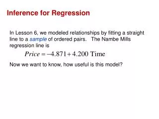
Inference for Regression. Chapter 14. The Regression Model. The LSRL equation is ŷ = a + bx a and b are statistics; they are computed from sample data, therefore, we use them to estimate the true y-intercept, α , and true slope, β μ y = α + β x

E N D
Inference for Regression Chapter 14
The Regression Model The LSRL equation is ŷ = a + bx a and b are statistics; they are computed from sample data, therefore, we use them to estimate the true y-intercept, α, and true slope, β μy = α + βx a and b from the LSRL are unbiased estimators of the parameters α and β
Testing Hypotheses of No Linear Relationship The null hypothesis H0 : β = 0 A slope of 0 means (horizontal line) no correlation between x and y. The mean of y does not change at all when x changes. The alternative hypothesis Ha: β≠ 0 or Ha: β < 0 or Ha: β > 0 Negative slope Positive slope
Testing Hypotheses of No Linear Relationship When testing the hypothesis of no linear relationship a t statistic is calculated In fact, the t statistic is just the standardized version of the least squares regression slope b. t = so we use table C to look up t and find the p-value. The P-value is still interpreted the same way.
b is the slope from the least squares regression line, SEb is the standard error of the least-squares slope b. SEb = Where s = And SEb = Therefore t = or t = t =
σ, the standard error about the LSRL (about y) is estimated by s = s =
Assumptions for Regression Inference • We have n observations of an explanatory variable x, and a • response variable y. Our goal is to predict the • behavior of y for given values of x. • For any fixed value x, the response y, varies • according to a normal distribution. • Repeated responses of y are independent of • each other. • The mean response μy has a straight line relationship with x. • μy = α + βx • α and β are unknown parameters • The standard deviation of y (call it σ) is the same for all values of x. • (σ is unknown)
Steps forTesting Hypotheses of No Linear Relationship • Make a scatter plot to make sure overall pattern of data is roughly linear (data should be spread uniformly above and below LSRL for all points) • Make a plot of residuals because it magnifies any unusual pattern (again, uniform spread of data above and below y=0 line is needed) • Make a histogram of the residuals to check that response values are normally distributed. • Look for influential points that move the regression line and greatly can greatly affect the results of inference.
Note: Minitab output always gives 2-sided p-value for Ha If you want the p-value for alternative hypotheses of Ha: β>0 or Ha: β< 0 just divide p-value from minitab by 2 Calculator gives you your choice
Confidence Interval for the Regression Slope βis the most important parameter in regression problem because it is the rate of change of the mean response as explanatory variable x, increases. CI for β b ± t* Seb estimate± t* SEb SEb = = t * look up on table C with n-2 degrees of freedom
Notes: You can also find CI for αsame way, using SEa a ± t*Sea (not commonly used)