Download

1 / 35
350 likes | 461 Vues
ECPC Seasonal Prediction System. Masao Kanamitsu Laurel DeHaan Elena Yulaeva and John Roads. Current model used. T62L28 Reduced grid MPI version running on 32 or 62 processors Time scheme Time splitting 30 min. time step. Physics. Relaxed Arakawa Schubert convection scheme. (S?)

E N D
ECPC Seasonal Prediction System Masao Kanamitsu Laurel DeHaan Elena Yulaeva and John Roads
Current model used • T62L28 Reduced grid • MPI version running on 32 or 62 processors • Time scheme • Time splitting • 30 min. time step
Physics • Relaxed Arakawa Schubert convection scheme. (S?) • M.D. Chou, long and short wave radiation. (S?) • Cloudiness based on RH. Further tuning by Meinke. (O) • Non-local PBL (S?) • Gravity wave drag by Alpert et al. (O?) • Smoothed mean orography from gtopo30. (S?) • NOAH land scheme with high resolution surface characteristics (N) • Leith horizontal diffusion on quasi-pressure level (S?) • Tiedtke shallow convection scheme (S?) • Surface pressure correction. (?) • SST surface angulations correction (S?) S: Same as NCEP SFM O: Older than NCEP SFM N: Newer than NCEP SFM
Timing • Total 134 months (11.2 years) • Ten 1-month AMIP + • Twelve 7-month • Ten 4-month • Using 30 processors (3GHz Xeon) • 38 hours (38 sec. per day)
ECPC Seasonal Forecast Predicted SSTs VanDenDool Predicted SSTs Ldeo Predicted SSTs NCEP ECPC SFM (8 hrs for each SST) 12 members 4 from each SST Observed SSTs, snow, and ice from NCEP AMIP (2 hrs) 7 months ECPC SFM (11 hrs) 4 months 10 members 1 month Persisted SST anomaly Times given are with 30 processors. With 60 processors, the entire forecast can be done in approximately 20 hours.
http://ecpc.ucsd.edu/projects/GSM_seasons.html GLOBAL ANOMALY PNA ANOMALY SPREAD CONSISTENCY
Performance comparisons FIG. 2. The weight values assigned to each model simulation by the revised six-model optimal combination scheme, for JAS precipitation. Weights , 0.01 are denoted by white. (Robertson et al., 2004)
A Comparison of the Noah and OSU LSMs used in 53 year AMIP runs ECPC has 2 sets of AMIP runs using our version of the NCEP GSM 1) 1949-2001, 10 member with OSU LSM 2) 1949-2001, 12 member with Noah LSM OSU LSM -The LSM created by Oregon State University in the 80’s which includes -thermal conduction equations for soil temperature -Richardson’s equation for soil moisture Noah LSM -Upgrade of the OSU LSM completed in 2002 which includes -increase from 2 to 4 layers -bare soil evaporation and thermal conductivity changes -frozen soil physics -snow melt changes -snow pack physics upgrade -treatment of thermal roughness
Noah – OSU 2m Temperature Difference for 1950-2000 Climatology Noah is generally warmer than OSU, especially in the wintertime high latitudes.
Noah – OSU Precipitation Difference for 1950-2000 climatology -The Noah LSM generally produces a greater amount of precipitation over land than the OSU LSM. -There is a shifting of precip over India and Indo-China in the summer.
Noah – OSU Anomaly Correlation Difference for 1950-1998 Overall, the skill between the two LSMs is similar. In the fall, the Noah LSM improves upon the OSU in most areas. Observations are from IRI.
ECPC’s Seasonal Forecast and Reanalysis-2 Verification SON Forecast from 200408 DJF Forecast from 200411 -Recently the Noah LSM replaced the OSU LSM. -Between Aug and Dec ’04, the forecast was run twice, once with each LSM.
The Ultimate Goal: Ensemble Long Lead Seasonal Forecasts of Climate Variables An example of the coupled model seasonal forecast of precipitation. The forecast integration was started in April 2005 http://ecpc.ucsd.edu/COUPLED/CM/coupled.html
Coupled modeling: approach • Goal: Coupled data assimilation model for seasonal (up to 12 months) climate prediction • Components: • ECPC Atmospheric Global Spectral Model • MIT Oceanic General Circulation Model (JPL version) • Initialization from consistent ocean and atmosphere states, coupling every 24 hours • Computationally effective coupling procedure
MIT Ocean General Circulation Modelhttp://www.ecco-group.org/ • Primitive equations on the sphere • ECCO package • GM eddy parameterization • Full surface mixed layer model • 360x224 (1°x1° horizontal resolution telescoping towards the equator to 1/3°) horizontal resolution with 46 vertical levels • Adjoint MIT model exists and is routinely used in JPL together with the forward model for 3D ocean state estimation
Computational Implementation of the MIT OGCM • Fully Parallelized • 2D decomposition • MPI message passing • LAPACK, BLAS, NETCDF • Tested on IBM SP, Linux clusters • Optimized for SIO PC Linux cluster (ROCKS 3.2)
Coupled Model Experiments 1. Long Run (currently 20+ years) – climatology 2. Retrospective forecast experiments • 12 months long runs starting the first day of every months for 11-year (1994-2004) time period . Skill of the model depending on leading time • Similar experiments but for the different initial month . Skill of the forecast depending on lead time and season. 3. Experimental Forecasts based on the climatology from retrospective forecasts
Global ROMS December JPL MIT: Jan.-Feb.-Mar. SST and surface flow for the Gulf Stream, Loop Current, & Labrador Current
Global ROMS December JPL MIT: Jan.-Feb.-Mar.
Skill of the long integration Spectra of the time series of the simulated and observed SST anomalies averaged over NINO3.4 region (5˚N-5˚S, 170˚W-120˚W). Both model and observations have picks in between 3 and 5 years
Skill of the El Nino Prediction Prediction skill of the coupled model. Correlation between the predicted and observed NINO 3.4 SST anomalies. The skill usually drops by the 4-th month, but then picks up after the coupled model dynamics starts to influence the predictability.
NINO3.4 simulation skill from the retrospective March forecasts Retrospective SST NINO3.4 forecast skill for the coupled model integration started in March (blue lines) compared to the reanalysis data (red line)Except for the 2002 integration, the simulated anomalies, closely follow the Reanalysis data.
11-months lead ocean forecast (from May 2005) Comparison between predicted (lower panel) and assimilated at JPL (upper panel) SST anomalies for JFM 1998. The coupled model run was started May 1-st, 1997. For “strong forcing” year, the model successfully predicts the main patterns of the SST anomalies for up to 11 months lead.
1998 JFM atmospheric forecast (from May 1997) Comparison between predicted Z500 (right panel) and Z500 from Reanalysis (left panel) for JFM 1998. The coupled model run was started May 1-st, 1997. The difference is much smaller than the response.
Forecast starts 3 months lead 6 months lead January 0.2 (AMJ) 0.1 (JAS) February 0.4 (MJJ) 0.1 (ASO) March 0.6 (JJA) 0.1 (SON) April 0.3 (JAS) 0.4 (OND) May 0.2 (ASO) 0.1 (NDJ) June 0.4 (SON) 0.3 (DJF) Skill of mid-latitude (170°E - 150°W; 45°N-65°N) Z500 prediction
SST Coupler every 24 hrs: Interpolation, integration Net heat, fresh water, SW radiation fluxes, wind stress. ECPC Coupled Experimental Seasonal Prediction Model Jet Propulsion Laboratory (JPL) version of the Massachusetts Institute of Technology (MIT)OGCM1°x1° with a telescoping 1/3° resolution close to the equator, 46 vertical levels.Adjoint model exists, routinely used in JPL for ocean state estimation Global Spectral ModelT62 (~200 Km) , 28 vertical levels Physical processes originated from NCEP-DOE reanalysis (R-2) Global and Regional versions are used for experimental seasonal climate predictions at ECPC Initial Conditions: JPL ocean assimilated data Initial Conditions: NCEP R-2
Experimental ECPC Coupled forecast The graph compares May forecast made by the ECPC Coupled model with forecasts made by other dynamical and statistical models for SST in the Nino 3.4 region for ten overlapping 3-month periods. The data for 'non-ECPC' models is obtained from IRI.
Summary • Experiment with the long run has shown that the current version of the coupled model produces realistic intrinsic variability. There is no drift, thus no flux adjustment is necessary. • The validation of the retrospective forecasts revealed that the skill of the model improves after a few months dew to coupling • The current ECPC NINO 3.4 SST forecast lies within the scatter of the IRI forecasts
Future plans • 2005-2006 • Implement cloud water prediction • Minor NOAH upgrade. • Single member coupled forecast • Experimental downscaling over western US • 2007-2009 • Implement VIC with tiling • Ensemble coupled forecast • Ensemble downscaling • 2010- • Ensemble coupled regional downscaling