Download
1 / 31
310 likes | 448 Vues
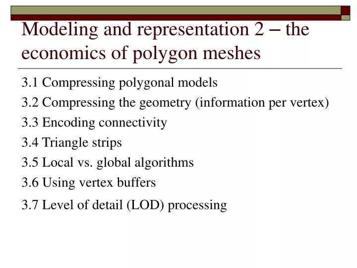
Modeling and representation 2 – the economics of polygon meshes. 3.1 Compressing polygonal models 3.2 Compressing the geometry (information per vertex) 3.3 Encoding connectivity 3.4 Triangle strips 3.5 Local vs. global algorithms 3.6 Using vertex buffers

E N D
Modeling and representation 2 – the economics of polygon meshes 3.1 Compressing polygonal models 3.2 Compressing the geometry (information per vertex) 3.3 Encoding connectivity 3.4 Triangle strips 3.5 Local vs. global algorithms 3.6 Using vertex buffers 3.7 Level of detail (LOD) processing
3.1 Compressing polygonal models • There are three ways of reducing the information per polygon • We can reduce the information sent the per polygon vertex • We can reduce the number of vertices, and the common way of doing this is to generate so called trip-strips for the polygon object. • We can reduce the number of polygons per object according to the number of pixels onto which it projects. This is called level of detail or LOD • Coarsening the numerical accuracy of geometric coordinates or colour values, are lossy. • Tri-strips, on the other hand, are lossless.
3.2 Compressing the geometry (information per vertex) • The minimum information required per vertex in a basic application if no compression techniques are adopted. An absolute minimum information set is : • (x, y, z) three-dimensional screen space coordinate of the vertex (12 bytes) • (u, v) texture (colour) coordinates (8 bytes) • (u, v) light map coordinates (8 bytes) • This can only be reduced further by sharing texture coordinates
3.2 Compressing the geometry (information per vertex) • The data volume can be reduced in most cases by encoding the difference between successive data items and some predicted value rather than their value. • Entropy reduction means encoding data items using a symbol whose bit length is inversely proportional to the frequency of occurrence of the data item in the application • Geometry and colour information can be further subject to both lossy and lossless compression techniques.
3.2 Compressing the geometry (information per vertex) • Deeirng(1995) suggests on the basis of empirical visual tests that the model’s local space specification should be restricted to 16 bits per component and then be subjected to delta compression or encoding. • Deering points out that the deltas of position components are not statistically uncorrelated.
3.2 Compressing the geometry (information per vertex) • Chow’s(1997) method also starts from a basis of bits per component but automatically finds the best quantisation (in the range 3 to 16 bits) for an object.
3.3 Encoding connectivity • We can consider ways of defining vertex connectivity in a mesh. • For example, a height field; conventionally used to represent terrain, the mesh connectivity is understood to be formed from a rectangular array. • We only need store the height of each vertex • For a general object, we specify a pointer for each vertex into an array of vertex positions.
3.3 Encoding connectivity • Assume that we have quantised the vertex components to 10 bits then for an object of n vertices we have: vertex cost = 30n bits • A theorem due to Euler shows that, in general, for a triangle mesh there are twice as many triangles as there are vertices. Thus we have, for a scheme where each triangle vertex points into a lost of n vertices: connectivity cost = bits and total cost =
3.3 Encoding connectivity • Rossingac(1999) suggests the following scheme which does not use explicit connectivity information and does not duplicate vertex data. • Each triangle has a vertex descriptor which is either the 30-bit vertex data or a pointer to an already encountered vertex. • A one-bit flag indicates which type of descriptor the vertex consists of • Again we have 6n elements in the structure but 5n of these are pointers to previous elements. The total cost now: vertex cost = (1+30)n bits pointer cost = (1+ )5n bits
3.4 Triangle strips • Triangle strips or tri-strips are a way of compressing the vertex connectivity information in a triangle mesh. • Tri-strips order triangles so that consecutive triangles share an edge, reducing the vertices per strip from 3n (if n triangles were sent separately ) to n+2 because it is only necessary to specify on new vertex per triangle. • An implementation of this method enables two consecutive vertices to be stored in a buffer which forms in effect a FIFO queue. • The class of meshes that con be represented by a sequential triangulation is very limited and the constraint can be relaxed by allowing two of the registers to be swapped.
3.4 Triangle strips • Examples
3.4 Triangle strips • Examples
3.5 Local vs. global algorithms • The first appearance of an algorithm for constructing tri-strips from meshes appears to be due to SGI (Akeley et al. 1990) • The algorithm constructs a path through the triangles by choosing a neighbour to the current triangle which is itself adjacent to the least number of (unvisited) neighbours. • If the algorithm encounters more than on triangle with the same least number of neighbours then it looks ahead on level and applies the same test.
3.5 Local vs. global algorithms • Evans et al. (1996) categorise the SGI approach as a local algorithm and introduce the concept of a global algorithm where they conduct a global analysis of a mesh using a technique they term patchification. • This approach depends on the observation that many polygon mesh models exhibit large areas which consist of connected quadrilaterals. • The algorithm is based on finding these patches and tern triangulating these row-wise or column-wise at a cost of 3 SWAPs per turn
3.6 Using vertex buffers • As we have already implied, tri-strips need to be made as long as possible to exploit their compression potential. • There have been many approaches to this problem and no one standard solution. • When a mesh produces a number of tri-strips, vertices from adjacent strips are reused and this leads to the obvious approach that vertices should be stored on graphics hardware memory to enable reuse locally. • This is exactly the approach taken in Deering(1995), Bar-Yehuda and Gotsman(1996), and Evans et al.(1996).
3.6 Using vertex buffers (Deering) • Uses a stack buffer of size 16 and allows random access to any vertex stored in the stack. • Connectivity information is now embedded in stack commands as follow: • 1 bit/vertex to indicate whether the vertex is to be read form the stack • 4 address bits/vertex for stacked vertices • 1 bit/(new) vertex to indicate whether the vertex is to be pushed onto the stack • 2bits/vertex to indicate how to continue • If each vertex is reused once then the cost is 11/2 bits/vertex (again assuming twice as many triangles as vertices)
3.6 Using vertex buffers (Bar-Yehuda and Gotsman(1996)) • Bar-Yehuda and Gotsman(1996) investigate the relationship between rendering time and buffer size and show that a buffer size of 12.72 suffices to generate a minimum sequence for any triangle mesh of n vertices in time n • Buffer size can be traded against rendering cost expressed as the number of vertices transmitted per mesh
3.6 Using vertex buffers (Bar-Yehuda and Gotsman(1996)) • A triangle mesh is converted into a representation that is sequence of stack commands of the from: • push(v) the vertex sent down the pipeline is pushed onto the stack • draw(v1,v2,v3) draw a triangle with vertices v1, v2 and v3. These will be stack indices – the vertices must already be in the stack • pop(k) pop the stack k times • The convert meshes into a sequence of stack commands the use a recursive procedure which relies on a well-known graph theory algorithm – the planar separator theorem.
3.6 Using vertex buffers (Bar-Yehuda and Gotsman(1996)) • Planar separator theorem • The theorem states that a class of graphs with n vertices have a separator (g(n),β) (1/2 ≤β<1), if for any graph G(V,E) vertices in the class V can be partitioned into three U, S and W such that no edge in E joins a vertex in U with a vertex in W, and • The class of planar graphs has a separator computable in O(n) time. • This means that such a graph can be split into three sub-graphs such that one separates the other in the way described.
3.6 Using vertex buffers (Bar-Yehuda and Gotsman(1996)) • Planar separator theorem examples • A simple recursive procedure
3.6 Using vertex buffers (Bar-Yehuda and Gotsman(1996)) • Planar separator theorem examples • Thus for the mesh in Figure the following sequence is generated:
3.7 Level of detail (LOD) processing • An important consideration in the discussion of LODs is smoothness of the on-screen transition from one level to another. • If the difference between successive LODs is large then there will be a popping effect on the screen • Another consideration is the selection of an appropriate level.
3.7 Level of detail (LOD) processing (Schroeder et al. in 1992 ) • A direct and simple approach for triangular meshes derived from voxel sets was reported by Schroeder et al. in 1992. • Here the algorithm considers each vertex on a surface
3.7 Level of detail (LOD) processing (Hoppe) • Hoppe (1996) gives an excellent categorisation of the problems and advantages of mesh optimisation, listing these as follows: • Mesh simplification • Reducing the polygons to a level that is adequate for the quality required (depends on the maximum projection size of the objection on the screen) • Level of detail approximation • A level is used that is appropriate to the viewing distance. • Construct smooth visual transitions, geomorphs , between meshes at different resolutions
3.7 Level of detail (LOD) processing (Hoppe) • Progressive transmission • Successive LOD approximations can be transmitted and rendered at the receiver. • Mesh compression • Analogous to two-dimensional image pyramids, we can consider not only reducing the number of polygons but also minimising the space that any LOD approximation occupies. • Selective refinement • A LOD representation may be used in a context dependent manner.
3.7 Level of detail (LOD) processing (Hoppe’s progressive mesh scheme) • Transition from a lower to a higher level: Vertex split • Transition from a higher to a lower level: Edge collapse
3.7 Level of detail (LOD) processing (Hoppe’s progressive mesh scheme)
3.7 Level of detail (LOD) processing (Hoppe’s progressive mesh scheme Notation) • Vf1 and Vf2 are two vertices in the finer mesh that are collapsed into one vertex Vc in the coarser mesh • where • From this diagram it can be seen that this operation implies the collapse of the two faces f1 and f2 into new edge • Continuum of geomorphs between the two levels by having the edge shrink under control of the blending parameter as : • d= • and (α is blending parameter)
3.7 Level of detail (LOD) processing (Hoppe’s progressive mesh scheme Notation) • Simple metric used to order the edges for collapse: • ( Vertex normals) • A more considered approach: • Energy Function minimization problem
3.7 Level of detail (LOD) processing (Energy Function minimization ) • Energy function to be minimized: • Orders all the legal edge collapse transforms into a priority queue. • An edge collapse is only legal it it does not change the topology of the mesh
3.7 Level of detail (LOD) processing • Simple edge elimination criterion