Download
1 / 9
90 likes | 94 Vues
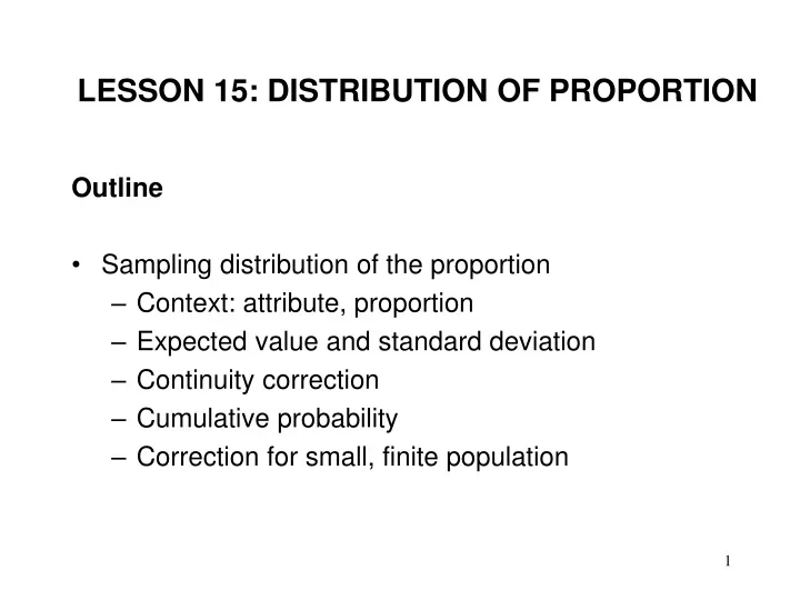
LESSON 15: DISTRIBUTION OF PROPORTION. Outline Sampling distribution of the proportion Context: attribute, proportion Expected value and standard deviation Continuity correction Cumulative probability Correction for small, finite population. SAMPLING DISTRIBUTION OF THE PROPORTION.

E N D
LESSON 15: DISTRIBUTION OF PROPORTION Outline • Sampling distribution of the proportion • Context: attribute, proportion • Expected value and standard deviation • Continuity correction • Cumulative probability • Correction for small, finite population
SAMPLING DISTRIBUTION OF THE PROPORTION • Context: Suppose that each item can have two states. The item either has an attribute or it does not. For example, an item can be either defective or not. • Usually, the states are good/bad, defective/non-defective, yes/no etc. • Sample proportion is used to draw inference about the unknown population proportion • Where is the number of sample observations having a particular attribute and is the sample size
SAMPLING DISTRIBUTION OF THE PROPORTION • Recall that binomial distribution applies in such cases. However, since the sample size is usually large, binomial distribution involves a large volume of computation. • A more convenient approach is to use the normal approximation to the binomial distribution. The expected value and standard deviation are computed as follows: • However, the binomial distribution of R (e.g., # of defectives) is discrete and the normal distribution is continuous. So, continuity correction may be required.
SAMPLING DISTRIBUTION OF THE PROPORTION • Continuity correction: • Binomial probability P(R=r) is approximated by normal probability P(r-0.5 R r+0.5) • This simple rule gives rise to many adjustments Binomial Normal P(R=r) P(r-0.5 R r+0.5) P(aR b) P(a-0.5 R b+0.5) P(R r) P(R r+0.5) P(R r) P(R r-0.5)
SAMPLING DISTRIBUTION OF THE PROPORTION • Summary: The cumulative probability is obtained as follows:
SAMPLING DISTRIBUTION OF THE PROPORTION Example 1: A welding robot is judged to be operating satisfactorily if it misses only 0.6% of its welds. A test is performed involving 50 sample weds. If the number of missed sample weds is more than 1, the robot will be overhauled. Find the probability that a satisfactory robot will be overhauled unnecessarily.
SAMPLING DISTRIBUTION OF THE PROPORTION • Correction for small population: The formula for standard deviation requires a little correction if the population is small. For small/finite population, the cumulative probability is obtained as follows:
SAMPLING DISTRIBUTION OF THE PROPORTION Example 2: A sample of 100 parts is to be tested from a shipment of 400 items altogether. Although the inspector does not know the proportion of defective in the shipment, assume that this quantity is 0.02. Determine the probability that
READING AND EXERCISES Lesson 15 Reading: Section 9-5, pp. 282-284 Exercises: 9-31, 9-32