Download
1 / 30
300 likes | 429 Vues
Dynamic Point Location via Self-Adjusting Computation. Kanat Tangwongsan Joint work with Guy Blelloch, Umut Acar, Srinath Sridhar, Virginia Vassilevska. Aladdin Center - Summer 2004. The Planar Point Location Problem. Classical geometric retrieval problem.

E N D
Dynamic Point Location via Self-Adjusting Computation Kanat Tangwongsan Joint work with Guy Blelloch, Umut Acar, Srinath Sridhar, Virginia Vassilevska Aladdin Center - Summer 2004
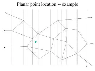
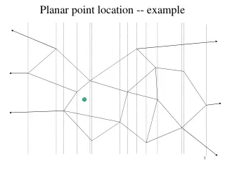
The Planar Point Location Problem • Classical geometric retrieval problem. • Subdivide a Euclidean plane into polygons by line segments. (These segments intersect only at their endpoints). • Identify which polygon the query point (red spot) is in.
Dynamic Point-location • insert, delete segments • query for point
Approaches • Approach I: dynamic by design • Usually complex, and cannot be composed together • Approach II: re-run the algorithm when input changes • Very simple • General • Poor performance • Approach III: smart re-execution • Identify the affected pieces and re-execute only the affected parts • More efficient. • Perhaps, takes only time proportional to the “edit distance”.
Smart re-execution in Point-Location • Identify point-location algorithms that are easily adapted to do “smart re-execution” efficiently. • Sarnak-Tarjan, 1986 • Simple and elegant • Idea: (partial) persistence • O(log n)-query-time, O(n)-space solution. • Static: unable to insert/delete segments • Equivalent to storing a “persistent” sorted set
Sarnak-Tarjan Ideas • Draw a vertical line through each vertex, splitting the plane into vertical slabs. Yield O(log n)-query time. (Dobkin-Lipton)
Sets of line segments intersecting contiguous slabs are similar. (Cole) • Reduces the problem to storing a “persistent” sorted set. A B
Our Work Dynamic Point-Location Algorithm Automatic Dynamizing Machine Sarnak-Tarjan • Build an efficient automatic dynamizing machine. • Analyze the efficiency of the resulting algorithm.
Smart Re-execution (revisited) • a.k.a. “self-adjusting computation” • Pioneer work by Acar et al (in SODA 2004) • Idea: keep track of who read what and when, so that as the input changes, we know exactly who to wake up to re-execute the affected area. • Extensions I worked on: • Previous version: order maintenance is O(log n) • The need for fast total order set of timestamps • New version is amortized O(1) • Previously, work only on purely functional program • Write-once
Closer Look: Order-Maintenance Problem • Maintain a list of records • Operations • insert (x, r) insert a new record r after x • delete (r)delete record r from the list • order (x, y) tells if x comes before y in the list • Naïve approach: use standard linked-list • Better tricks? • Dietz, Tsakalidis, Dietz-Sleator, Bender et al. b l y a q r p t x
Closer Look: Order-Maintenance Problem(cont.) • Dietz-Sleator, 1987 • Amortized O(log n) algorithm for insert and O(1) for delete/order. • Label each record with a special tag • Size limit at for n-bit machine • Explain the use of two-level constructions to achieve O(1) • Bender et al, 2002 • Same doubly linked-list idea • Achieve similar bounds • Less constrained on size • Also suggest the possibility to achieve O(1) bounds
Our Solution • Hybrid • Two levels: Dietz-Sleator’s construction • Bender’s for each list (each list is circular, and doubly linked) • Top level contains pointers to the child-level lists • Split the child-level list in half, if #nodes exceeds the constant c (on an n-bit machine, c ~ n) Top-level Child-level x y
Running Time • order/delete: obvious worst-case O(1) • insert: • c is chosen to be roughly logN, N = largest integer. • Intuitively: each ring has ~ log n, n = #records • Since the child ring is small, the bottom level is no big deal. • Roughly, there are top-level nodes • Thus, spending per log n insertions
Other Changes • Revised interface: support imperative program • Experiment on merge sort, insertion sort, quick sort, graham scan (convex hull), etc. • (in progress) design new techniques for multiple writes to each location. • Naturally occur in imperative settings
Review: Skip Tree • Skip-list • Alternative to balanced search tree – same O(log n) bound • Allow searching in a totally ordered set of keys • Skip tree [see Motwani-Raghavan Randomized Algorithms] • Unique path between any two nodes • Each right pointer ends at the tallest node of the key 7 1 ! 7 1 6 ! ! 0 1 9 3 6 7 7 1 2 4 5 8 3 6 9 0 !
Simplified Point-Location • Only horizontal lines (x1, x2, y) • Given q = (x*, y*), find the closest line above that point. • In persistent sorted set, • Line (x1, x2, y) means insert y at time x1 and delete it at x2 • To look up q = (x*, y*), do a search at timex* • Previous work shows • Equivalent to the original planar point-location problem
Running Sarnak-Tarjan • I = the set of segments i.e. input • A = our Sarnak-Tarjan algorithm (using skip tree) • The execution of A on I is a series of insert/delete at various time. p q r
Re-execution • I * = the set of segments differing from I by one segment • For ease, I * = I + {s}, where s = (x1, x2, y) is a segment. • So, p q r s Insert s Delete s
An Illustration p q r s
Observations • Recall: each consists of a search • Each search path is a sequence of visited nodes. • Same search paths except for
d i i+d Lemma A: Ancestor relationship • Consider a skip tree with ordered set of keys {1, 2, …, n} • Pr [i is on the path to i+d] = (1/d).
Lemma A: Ancestor relationship(cont.) • Consider a skip tree with ordered set of keys {1, 2, …, n} • Pr [i is on the path to i+d] = (1/d). • Proof: • level of the keys in between · that of i • Level of each key is independent of one another • Thus, i i+d
Lemma B: Difference in search-path • Consider a search to the key y* (any key) • Same path unless happening between Is and Ds • The difference is expected (1/d), where d = #keys between y and y* A(I*) A(I) Old World New World y y* y*
Cost A Cost B y* y Lemma B (cont.) Cost A • Let V = #nodes with key y visited • Pr[V = m] • = Pr[V = m|visit y]£Pr[visit y] • = 2-m £(1/d) • Cost A = E[V] = (1/d) Cost B • Proof omitted • Yield same (1/d)
Summary • Lemma B gives an immediate lower-bound for point-location in this framework. where y’ is the y’s of those lines overlapping with y, and d(y, y’) = #lines in between y and y’ (when searching for y’) • Close to match this bound • Introducing partial path-copying and probability node copying