Download
1 / 12
120 likes | 318 Vues
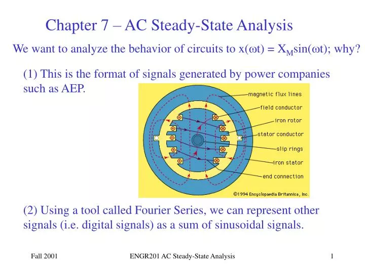
Chapter 7 – AC Steady-State Analysis. We want to analyze the behavior of circuits to x( t) = X M sin(t); why?. (1) This is the format of signals generated by power companies such as AEP.

E N D
Chapter 7 – AC Steady-State Analysis We want to analyze the behavior of circuits to x(t) = XMsin(t); why? (1) This is the format of signals generated by power companies such as AEP. (2) Using a tool called Fourier Series, we can represent other signals (i.e. digital signals) as a sum of sinusoidal signals. ENGR201 AC Steady-State Analysis
XM 2 /2 3/2 t -XM t T x(t) = XMsin(t); The function is periodic with period T x[(t+T)] = x(t ) Frequency, f, is a measure of how many periods(or cycles) the signal completes per second and is measured in Hertz (cycles per second ) is the angular frequency and is measured in radians per second ENGR201 AC Steady-State Analysis
sin(120t) sin(120t- /4) Phase Shift - a sinusoid can be shifted right (left) by subtracting (adding) a phase angle. x(t) = XMsin(t + ) Note that one function lags (leads) the other function of time. ENGR201 AC Steady-State Analysis
sin(120t+ /4) ENGR201 AC Steady-State Analysis
Some useful trigonometric identities: Multiple-angle formulas: ENGR201 AC Steady-State Analysis
Sinusoidal & Complex Forcing Functions R v(t)=VMcost i(t) L If we apply sinusoidal signals (voltages and/or currents) as inputs to linear electrical networks, all voltages and currents in the circuit will be sinusoidal also; only the amplitudes and phase angles will differ. The following example illustrates. ENGR201 AC Steady-State Analysis
R v(t)=VMcost i(t) L Let us assume (this is a theorem from differential equations) that the solution to the differential equation, i(t), is also sinusoidal. That is, the forced response can be written i(t) = Acos(t+) The signal has the same frequency, but different magnitude and phase. However, this expression must satisfy the original differential equation. ENGR201 AC Steady-State Analysis
R v(t)=VMcost i(t) L i(t) = Acos(t+ ) Using the multiple angle formula: i(t) = Acostcos - Asin tsin i(t) = A1 cost + A2 sint ENGR201 AC Steady-State Analysis
Setting like terms on each side of the equation equal yields two simultaneous equations: Solving these two simultaneous equations yields: Since i(t) = A1 cost + A2 sint ENGR201 AC Steady-State Analysis
Using trig identities we get: Conclusion: we do not want to use differential equations to analyze such circuits! ENGR201 AC Steady-State Analysis
Euler’s Identity We can write our sinusoidal forcing functions in terms of the complex quantity ejt v(t) = VMcost = Re[VMejt] = Re[VMcost + j VMsint ] The currents and voltages produced can also be written in terms of ejt i(t) = Imcos(t +) = Re[Imej(t + )] i(t) = = Re[Imcos(t +) + j Imsin(t +) ] Using complex forcing functions allows us to use (complex) algebra in place of differential equations. ENGR201 AC Steady-State Analysis
R v(t)=VMejt i(t) L i(t) = Imej(t +) ENGR201 AC Steady-State Analysis