Download
1 / 73
780 likes | 1.08k Vues
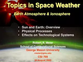
Topics in Space Weather Lecture 12. Ionosphere. Robert R. Meier School of Computational Sciences George Mason University rmeier@gmu.edu CSI 769 22 November 2005. Topics. Photoionization & Photoelectrons Photoionization & Chapman Layer Ionospheric Layers F-Region E-Region D-Region

E N D
Topics in Space WeatherLecture 12 • Ionosphere Robert R. Meier School of Computational Sciences George Mason University rmeier@gmu.edu CSI 769 22 November 2005
Topics • Photoionization & Photoelectrons • Photoionization & Chapman Layer • Ionospheric Layers • F-Region • E-Region • D-Region • Ionospheric Regions • Equatorial • Midlatitudes • High Latitudes
Photoionization and Photoelectrons Important source of Secondary ionization Dayglow emissions Heat source for plasmasphere Conjugate photoelectrons important Concepts analogous to auroral electron precipitation
Photoionization Processes • O + h ( 91.0 nm) O+ + e • O2 + h ( 102.8 nm) O2+ + e • N2 + h ( 79.6 nm) N2+ + e Ionization Energies
Photoelectron Energy • Example: Ionization of O by solar He+ emission at 30.4 nm • Photon energy: Es (eV)= hs = hc/s = 12397/304 = 40.78 eV • Ionization into ground state of O+ • Ionization potential is 13.62 eV • Excess energy: E = Es - EIP = 40.78 – 13.62 = 27.16 eV • What happens to excess energy? Kinetic energy of photoelectron S = Sun PE = photoelectron IP = ionization potential
Photoelectrons, cont.What about ionization into excited states of ions? • O(4S): 13.62 eV • Ground state of ion • O(4P): 28.49 eV • First allowed state • He+ Photon can ionize into 4P state: 28.49 eV < E30.4 = 40.78 eV • Kinetic energy of photoelectron: 40.78 – 28.49 = 12.29 eV Ground state of atom From Rees, Phys. Chem. Upper Atmos.
Photoelectrons, cont. • Photoelectrons produced when O+ is in the ground state have sufficient energy to ionize O • EPE = 28.49 eV > 13.62 eV (ionization potential of O) • Note that if O+ is in the 4P state, the excess energy is 12.29 eV • Not sufficient to ionize N2 or O, but is for O2 • Therefore photoelectrons are an important source of secondary ionization • ~25% at higher altitudes • More at lower altitudes where X-rays can produce very energetic photoelectrons
Photoelectrons, cont. Full computation of photoelectron flux requires solution of Boltzmann transport equation • Production • Photoionization into ground and excited states of N2+, O2+,O+,N+ • Secondary ionization by energetic photoelectrons • Doubly ionized species not significant • Loss • Elastic scattering • Scattering by neutrals • Coulomb collisions • Inelastic scattering • Ionization • Excitation of electronic, vibrational, rotational states • Dissociation • Transport
Photoelectrons, cont. Dominant Energy Losses: EPE > 50 eV: ionization and excitation of atoms and molecules EPE ~ 20 eV: excitation of atoms and molecules EPE < 5 eV: excitation of vibrational states of N2 EPE < 2 eV: coulomb collisions with ambient electrons
Photoelectrons, cont. • Full solutions of Boltzmann equation • Mantas [Plan. Space Sci, 23, 337, 1975] • Oran and Strickland [Plan. Space Sci., 26, 1161, 1978] • Link [J. Geophys. Res., 97, 159, 1992] • Simpler approach • Richards and Torr [J. Geophys. Res., 90, 2877, 1985]
Photoelectron Flux • Following Richards and Torr, ignore • Transport • Coulomb collisions • Cascade of high energy photoelectrons to lower energy photoelectrons • EPE < 20 eV • O2 • Simple Production = Loss gives insight into photoelectron flux spectrum
Photoelectron Flux • Production qN2(z,E) = nN2(z)Fs(z,E()) (E) dE nN2(z) I(E) exp(- eff(z,E)) Similar expression for O • Loss LN2 = (z,E) N2(E) nN2(z) = photoelectron flux (PE cm-2s-2 eV-1) N2 = total energy loss cross section for e*+N2 collisions
Photoelectron Flux Production = Loss or qtotal = Ltotal nN2(z) IN2(E) exp(- eff(z,E)) + nO(z) IO(E) exp(- eff(z,E)) = (z,E) N2(E) nN2(z) + (z,E) O(E) nO(z) Solving for :
Photoelectron Flux, cont. If then and the photoelectron flux • altitude dependence is from the effective attenuation of the solar flux • energy dependence is from the production frequency and energy loss cross section ratio • is independent of composition
Photoelectron Flux, cont. Simple and full PE flux calculations Some differences < 20 eV and > 50 eV Richards and Torr [1983]
Photoelectron Flux, cont. Simple and full PE flux calculations Compare with AE-E PE measurements Richards and Torr [1983]
Altitude Dependence of Photoelectron Flux Full PE flux calculations Note small change in energy shape with altitude - Supports Richards and Torr simple concepts
Photoelectron Energy Distribution Function Structure due To He+ 30.4 nm Thermal Electrons Photoelectrons
Photoionization • Example: O + h O+ + e*, … • Photoionization Frequency j(z) = Fs(z,) () d (# s-1) Fs(z,) = Fs(,) e-(z,) (photon cm-2 s-1 nm-1) () = photoionization cross section no(z) = O number density
Photoionization Rate • q(z) = no(z) j(z) (# cm-3 s-1) • no(z) = O number density • Assume single constituent, isothermal atmosphere, photoionized by a single wavelength emission: n(z) = no(z) = no(zo) e-(z-zo)/H q(z) = no(zo) e-(z-zo)/H Fs(,) e-(z,)
Photoionization Rate cont. Peak in layer occurs when Working through, this occurs at
Photoionization Rate cont. Substituting and rearranging terms leads to: For Sun at zenith, s
Recombination • Radiative Recombination O+ + e O + h • Recombination Coefficient • = 1.2 x 10⁻¹² (1000/T)1/2 cm-3 s-1 • Electron loss rate L(z) = nO+(z) ne(z) = ne2(z)
Chapman Layer Production = Loss (Steady-state: dne/dt =q-L = 0) q(z) = L(z) = ne2(z) Solving for the electron density ne(z) = [q(z) / ]1/2 or s = 80 0 60 40
Ionospheric Layers D-Region E - region F1 – Region F2 – Region Plasmasphere
Ionospheric Layers Similar to Chapman Layers F2 F1 Total ne E
D-Region • Ugly ion chemistry • See: • Turunen, E., H. Matveinen, J. Tolvanen, and H. Ranta, D-region ion chemistry model, in STEP Handbook of Ionospheric Models, R. W. Schunk (ed.), pp. 1-25, 1996. • Torkar, K. M., and M. Friedrich, Tests of an ion-chemical model of the D- and lower E-region, J. Atm. Terr. Phys., 45, 369-385, 1983. • Tens of species—some models have more • Few measurements • Requires rockets
D-Region Chemical Scheme From Torkar, K. M., and M. Friedrich, 1983
Example Comparison of D-region Observations and Model From Torkar, K. M., and M. Friedrich, 1983
E-region • Production--photoionization O2 + h O2+ + e j = photoionzation rate N2 + h N2+ + e O + h O+ + e (smaller) • Chemistry • N2+ + O NO+ + N or O+ + N2 • O+ + N2 NO+ + N • Loss—Dissociative Recombination • NO+ + e N + O • O2+ + e O + O kO2+ = recombination rate • Net Result: • Major ions in E region are O2+ and NO+ • To first order, diffusion & dynamics slow compared with photochemistry
Electron Density in Lower Part of E-Region • O2+ is dominant ion • Ignore dynamics, diffusion
Electron Density in Lower Part of E-Region, cont. In steady state,
Recombination Rates and Electron Lifetimes Lower E-Region • O2+ + e O + O kO2+ = 1.9 x 10⁻⁷ (Te/300)-0.5 cm3s-1 • nO2+ ~ 105 cm-3 & Te ~ Tn = 300K at ~ 110 km • Rate = kO2+ nO2+ = 0.019 s-1 • Lifetime = 1/Rate = 53 s Upper E-Region • NO+ + e N + O kNO+ ~ 4.2 x 10⁻⁷ (Te/300)-0.85 cm3s-1 • nNO+ ~ 105 cm-3 & Te ~ Tn = 587K at ~ 140 km • Rate = kNO+ nNO+ = 0.024 s-1 • Lifetime = 1/Rate = 42 s
F1-Region • Similar to E-region • Must include O+, the dominant ion • Diffusion begins to be important
F2 Peak Region- Assume photochemical equilibrium - Ignore transport and diffusion F2-region ion chemistry rates O+ balance yields: jO nO = kN2 nN2 + kO2 nO2 Ignoring O2 in the upper ionosphere yields:
Important Result when Chemistry Dominates: ne nO/nN2 • Problem: As z increases, nN2 decreases much more rapidly than nO • Therefore ne exponentially as z increases • Solution • Transport becomes faster at high altitudes • Also at other times when electrodynamics become important
Recombination Rates and Electron Lifetimes in F-Region • Production: O + h O+ + e • Rate = j = 2 – 6 x 10⁻⁷ s-1 • Lifetime = 5 – 1.6 x 10⁶ s ( 58 - 19 days) • Intermediate step: O+ + N2 NO+ + N • (or O2) • Rate for N2: kN2 nN2 = 10-12cm3s-1 5.5x108cm-3 = 5.5 x 10⁻⁴ s-1 • Lifetime = 1800 s • Loss: NO+ + e N + O • ne ~ 106 cm-3 & Te ~ 1800K at ~ 250 km • Rate = kNO+ ne = 0.129 s-1 • Lifetime = 1/Rate = 7.8 s • Loss: O+ + e O • ne ~ 106 cm-3 & Te ~ 1400K at ~ 250 km • Rate = kO+ ne = 1.2x10⁻¹² (1000/T)0.5 x ne s-1 = 1 x 10⁻⁶s • Lifetime = 1/Rate = 106 s = 11 days
Simplified Ambipolar Diffusion • Electrons diffuse more rapidly than ions (initially) • Slight charge separation produced strong electric field • Ions “feel” electric field (E) and are pulled along by electrons to ensure charge neutrality
Ambipolar Diffusion, cont. • Again, diffusive equilibrium • net diffusion velocity is zero • Ignore ion chemistry • Assume plasma flow parallel to magnetic field lines • taken to be vertical (upper mid to high latitudes) • Assume single ion species • Same as neutral species • Note: can be generalized to multiple ions
Ambipolar Diffusion, cont. • Force on ions and electrons: Fi = eE (upward pull) Fe = - eE (downward pull) • Force balance for ions and electrons in slab of area, A: Ions: dpi A = - ni mi g Adz + ni eE Adz Electrons: dpe A = - ne me g Adz - ne eE Adz
Ambipolar Diffusion, cont. or and
Ambipolar Diffusion, cont. Gombosi, Equation 10.48
Ambipolar Diffusion, cont. • If Te = Ti = Tn, then (Assuming mi=mn) • Thus the ion scale height is twice the neutral scale height • The ion density profile is then: • More complete physics requires numerical solutions of differential equations
F-region Diffusion Times Atmosphere: from Homework 1 • Plasma Diffusion time: • D = Hi2 / Din • Din ~ 1x10¹⁹ / nn(Banks and Kockarts, Aeronomy) • Chemical lifetime: • C =(kN2 nN2)-1 (from slide 24) D C Diffusion is faster above 280 km and chemistry is, below See Section 7.5 of Tascione
Plasmasphere • Top of ionosphere • Strong interactions with magnetosphere, esp. during geomagnetic storms • Consider simple processes only • More complicated interactions with magnetosphere Add fig 10.7 from Gombosi
Plasmasphere, cont. • Photochemical equilibrium • Near resonant charge exchange O+(4S) + H(2S) O(3P) + H+E • E = EIP(O) - EIP(H) = 13.618 - 13.598 = 0.02 eV • Source and sink of H+ • Assuming photochemical equilibrium • As altitude increases, H/O increases, and H+ becomes the dominant ion Gombosi, 10.6
Plasmasphere, cont. • He+ is second most populous ion • Tracks He+ • Can image plasmasphere by observing resonant scattering of solar He+ 30.4 nm emission line He+(2S)+ h30.4 He+ (2P) He+(2S)+ h30.4 From IMAGE Satellite Sun