Download

1 / 38
380 likes | 462 Vues
M onoton ic relationship of two variables, X and Y. Deterministi c monotoni city. Y. 16. If X grows then Y grows too. 12. 8. 4. 0. X. 0. 1. 2. 3. 4. Stochasti c monotoni city. Y. 16. *. *. If X grows then likely Y grows too. *. 12. *. *. *. 8. *. *. *.

E N D
Deterministic monotonicity Y 16 IfX grows then Y grows too 12 8 4 0 X 0 1 2 3 4
Stochastic monotonicity Y 16 * * IfX grows then likely Y grows too * 12 * * * 8 * * * 4 * * * * * * * * 0 X 0 1 2 3 4
An example SsXY 1 1 35 2 1.5 34 3 2 36 4 3 37 5 7 38 6 10 39
Rank data separately for X and Y SsXrankYrank 1 1 1 35 2 2 1.5 2 34 1 3 2 3 36 3 4 3 4 37 4 5 7 5 38 5 6 10 6 39 6
Spearman-s rank correlation (rS):Correlationbetween ranksIn the above example: r = 0.91, rS = 0.94
Concordancy Discordancy
Concordancyand discordancy Y B + C - A X D
Kendall-stau p+: Proportion of concordant pairs in the population p-: Proportion of discordant pairs in the population t = p+ - p-
Features of Kendall’st • -1 £t£ +1 • If X and Y are independent:t= 0 • t = 0: no stochastic monotonicity • t = -1 (t = +1): deterministic monotonedecreasing (inreasing)relationship
A Kendall’s gamma For discrete X and Y variables
Features of Kendall’sG • -1 £G £ +1 • If X and Y are independent:G = 0 • G = 0: no stochastic monotonicuty • IfG = -1: p+ = 0 • IfG = +1: p- = 0
Testingthe H0: t = 0 null hypothesis • Sample tau: Kendall’s rank correlationcoefficient (rt) • Testingstochastic monotonicity = testing the significancy of rt
Computation of sample tau Y B c = n+ = 4 d = n- = 2 rt = (4-2)/(4+2) = 2/6 = 0.33 + + C C + + A - - D X
Formulea of rtandG c = # of concordancies d = # of discordancies T = # of total couples = n(n-1)/2 rt = (c - d)/T,G = (c - d)/(c+d) In which caseswill rt = G?
An example r= 0.91 (p < 0.02); rS= 0.94 (p < 0.02); rt = 0.84 (p < 0.10); SsXY 1 1 35 2 1.5 34 3 2 36 4 3 37 5 7 38 6 10 39
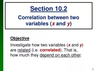
80 60 40 20 GSR-decrease 0 -20 -40 -60 Agr1 Agr2 Agr3 Light Verbal Groups
Average Rorschach time (min) 2.5 2 1.5 1 0.5 0 Normal Person.disorder Holocaust group
Comparison of population means H0: E(X1) = E(X2) = ... = E(XI) H0: m1 = m2 = ... = mI
Basic identity SStotal = SSb + SSw SStotal: Total variability SSb: Between sample variability SSw: Within sample variability
One-way ANOVA Varb = SSb/(I-1) = SSb/dfb - Treatment variance Varw = SSw/(N-I) = SSw/dfw - Error variance Test statistic: F = Varb/Varw
H0: m1 = m2 = ... = mI + Assumptions of ANOVA F = Varb/Varw ~ F-distribution F ³ Fa: reject H0at level a
Assumptions of ANOVA • Independent samples • Normalityof the dependent variable • Variance homogeneity (identical population variances)
Robust ANOVA’s • Welch test • James test • Brown-Forsythe test
Testing variance homogeneity • Levene test • O’Brien test
Trust in the result of ANOVA Var1» Var2» ... » VarI or (and) n1» n2» ... » nI
When to apply a robust ANOVA? • Different sample sizes • Substantially different sample variances
Post hoc analyses Hij: mi = mj • Conventional test:Tukey-Kramer test (Tukey’s HSD test) • Robust test:Games-Howell test
Nonlinearcoefficient of determination SStotal = SSb + SSw Explained variance: eta2 = SSb/SStotal Nonlinear correlation coefficient: eta
x i An example Agr Agr Agr Light Verb. 1 2 3 5 4 6 4 4 n i 14.50 6.75 5.20 -13.45 -30.08 s 29.60 9.15 6.96 13.11 14.57 i
Testing variance homogeneity • Levene test: • F(4, 7) = 0.784 (p > 0.10, n.s.) • O’Brien test: • F(4, 8) = 1.318 (p > 0.10, n.s.)
ConventionalANOVA Treatment var.: Varb = 1413.9 Error variance: Varw = 286.2 F(4, 18) = 1413.9/286.2 = 4.940** Nonlinear coeff. of determin.: eta2 = SSb/SStotal = 0.523
Robust ANOVA’s • Welch test: • W(4, 8) = 5.544* • James test: • U = 27.851+ • Brown-Forsythe test: • BF(4, 9) = 5.103*
Pairwise comparison of means Tukey-Kramer test: T12= 0.97 T13= 1.28 T14= 3.48 T15= 5.55** T23= 0.20 T24= 2.39 T25= 4.35* T34= 2.42 T35= 4.57* T45= 1.97