Download
1 / 25
250 likes | 357 Vues
Non-Gaussian Statistical Timing Analysis Using Second Order Polynomial Fitting. Lerong Cheng 1 , Jinjun Xiong 2 , and Lei He 1 1 EE Department, UCLA *2 IBM Research Center Address comments to lhe@ee.ucla.edu

E N D
Non-Gaussian Statistical Timing Analysis Using Second Order Polynomial Fitting Lerong Cheng1, Jinjun Xiong2, and Lei He1 1EE Department, UCLA *2IBM Research Center Address comments to lhe@ee.ucla.edu *Dr. Xiong's work was finished while he was with UCLA. This work was partially sponsored by NSF and Actel.
Outline • Background and motivation • Second order polynomial fitting for max operation • Quadratic SSTA • Experiment results • Conclusions and future work
Background and Motivation • Gaussian variation sources • Linear delay model, tightness probability [C.V DAC’04] • Quadratic delay model, tightness probability [L.Z DAC’05] • Quadratic delay model, moment matching [Y.Z DAC’05] • Non-Gaussian variation sources • Non-linear delay model, tightness probability [C.V DAC’05] • Linear delay model, ICA and moment matching [J.S DAC’06] • Non-linear delay model, Fourier Series [Cheng DAC’06] • Need fast and accurate SSTA for Non-linear Delay model with Non-Gaussian variation sources
Outline • Background and motivation • Second order polynomial fitting for max operation • Quadratic SSTA • Experiment results • Conclusions and future work
Linear Fitting: Tightness Probability • Previously, max operation is approximated by tightness probability [Chandu DAC04] where • Tightness probability approximation is a linear fitting • Tightness probability is hard to obtain when A and B are non-Gaussian random variables • Max operation is a non-linear operation • Linear fitting is not accurate enough • Need a more accurate and efficient non-linear approximation
Non-linear fitting of Max: Second Order Polynomial Fitting • Using second order polynomial instead of linear function to approximate the max operation where and V is a random variable with any arbitrary distribution • Fitting coefficients are computed by matching the mean of the max operation while minimizing the square error between h and max(V,0) within the 3σrange where How to obtain these Fitting Coefficients?
Mean of the Max Operation • When V is a non-Gaussian random variable, it is hard to compute E[max(V,0)] • Two step solution • We approximate the non-Gaussian random variable V as a quadratic function of a standard Gaussian random variable W by matching the first 3 moments [Zhang’ISPD05] • c2, c1, and c0 can be computed by close form formulas • Use E[max(g(W), 0)] to approximate E[max(V,0)]
Compute Fitting Coefficients • Recall the constraint that matching the mean of the max operation we have • The constrained optimization equation can be written as the unconstrained optimization equation: where • Expanding the integral, the square error can be represented as quadratic form of can be computed easily by letting partial derivative of SE to be 0
Comparison between Second Order Fitting and Linear Fitting • Assume V~N(0.7, 1)
Outline • Background and motivation • Second order polynomial fitting for max operation • Quadratic SSTA • Experiment results • Conclusions and future work
Quadratic Delay Model • Delay is quadratic function of variation sources • Xi’s are independent random variables with arbitrary distribution • Xi’s are with zero mean and unit standard deviation • R is local random variation, which is modeled as a Gaussian random variable
Atomic Operations for SSTA • Two atomic operations for block based SSTA, max and add • Given • Compute
Max Operation Flow Compute mean, variance, and skewness of Dp=D1-D2 Obtain the fitting coefficients Θ for max(Dp,0) Reconstruct Dm=max(D1,D2) to quadratic delay form
Moments of Dp • Quadratic form of Dp where • First three moments of DP • Because Dp is in quadratic form of variation sources Xi’s, the moments of Dp can be computed by close form formulas • With the first three moments, it is easy to obtain the fitting coefficients Θ for max(Dp,0)=h(Dp,Θ)
Reconstruct Dm to Quadratic Form • Fitting result of Dm • Dm is a 4th order polynomial of Xi’s • Moment Matching [Zhan DAC2005] • Joint moments between Dm and Xi’s can be computed by close form formulas
Add Operation • Just add the correspondent parameters to get the parameters of Ds
Computational Complexity • The computational complexity of one step max operation is O(n3), where n is the number of variation sources • The computational complexity of one step add operation is O(n2) • The complexity measured as the total number of max and add operations of the SSTA is linear with respect to the circuit size
Semi-Quadratic SSTA • Effect of the crossing terms in the quadratic model is weak [Zhan DAC2005], ignoring crossing terms will not affects the accuracy too much • Simplified delay model without crossing terms (semi-quadratic delay model) Where • The SSTA flow for the semi-quadratric delay model is similar to that of the quadratic delay model, but much simpler • The computational complexity of both max and add operation for semi-quadratic SSTA is O(n)
Outline • Background and motivation • Second order polynomial fitting for max operation • Quadratic SSTA • Experiment results • Conclusions
Experiment Setting • ISCAS89 benchmark set • 65nm technology • Two types of variation sources, both with skew-normal distribution • Leff • Vth • Three types of variation • Inter-die variation • Intra-die spatial variation (grid based model) • Intra-die random variation • Three comparison cases • Linear SSTA [Chandu DAC2004] • Nonlinear SSTA using Fourier Series [Cheng DAC2007] • 100,000 sample Monte-Carlo simulation
Error and Run Time Comparison • For quadratic SSTA, the error of mean, standard deviation, and skewness is within 1%, 1%, and 5%, respectively. • For Semi-Quadratic SSTA, the error of mean, standard deviation, and skewness is within 1%, 2%, and 25% error. • Semi-quadratic SSTA ignores crossing terms which affects skewness • Semi-quadratic SSTA results similar error as Fourier SSTA, but 20X faster • Semi-quadratic SSTA is more accurate than linear SSTA with similar run time
Outline • Background and motivation • Second order polynomial fitting for max operation • Quadratic SSTA • Experiment results • Conclusions
Conclusion • A new second order polynomial fitting of the max operation is proposed • All the SSTA operations are based on close form formulas • The quadratic SSTA predicts the error of mean, standard deviation, and skewnss withing 1%, 1%, and 5% error, respectively • The semi-quadric SSTA has similar accuracy as the SSTA with Fourier Series, but 20X faster