Download
1 / 42
620 likes | 1.59k Vues
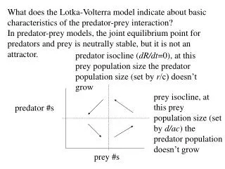
Lotka-Volterra, Predator-Prey Model. J. Brecker April 01, 2013. Alfred Lotka & Vito Volterra. Lotka (1880-1949). Volterra (1860-1940). Predator-Prey Model Assumptions. The Lotka-Volterra predator-prey model makes a few important assumptions about the

E N D
Lotka-Volterra, Predator-Prey Model J. Brecker April 01, 2013
Alfred Lotka &Vito Volterra Lotka (1880-1949) Volterra (1860-1940)
Predator-Prey Model Assumptions The Lotka-Volterra predator-prey model makes a few important assumptions about the environment and the dynamics of the predator and prey populations: 1. The prey population finds ample food at all times. 2. In the absence of a predator, the prey grows at a rate proportional to the current population; thus dx/dt = αx, α>0, when y=0. 3. The food supply of the predator population depends entirely on the prey populations. 4. In the absence of the prey, the predator dies out; thus dy/dt = - βy, β>0, when x=0.
Predator-Prey Model Assumptions 5. The number of encounters between predator and prey is proportional to the product of their populations. Encounters between predator and prey tends to promote the growth of the predator and inhibit the growth of the prey. Thus, the growth rate of the predator is increased by the term γxy and the growth rate of the prey is decreased by the term – δxy. 6. During the process, the environment does not change in favor of one species and the genetic adaptation is sufficiently slow.
Rabbits & Foxes Let, x(t): rabbit (prey population) @ time t. y(t): fox (predator) population @ time t.
The General Model Based on the assumptions for this model we have the following two-equation system of autonomous, first-order, nonlinear differential equations: • dx/dt = αx – δxy = x(α – δy), • dy/dt = – βy + γxy = y(– β + γy); α, β, δ, γ > 0.
The Parameters α: the growth rate of the prey β: the death rate of the predator δ, γ: measure the effect of the interactions of the two species
When (y = 0), equation (1) becomes: (3) dx/dt = αx – δxy = αx. dx/dt – αx = 0.
The general solution to equation (3) dx/dt – αx = 0 is: (4) x(t) = ceαt So, the rabbit (prey) population will increase exponentially in the absence of a predator.
Likewise, in the absence of a prey (x = 0), equation (2) becomes: (5) dy/dt = –βy + γxy = – βy. dy/dt + βy = 0. The general solution to this equation is: (6) y(t) = ce-βt The fox population will experience exponential decay until extinction in the absence of prey.
The Predator-Prey Model (1) dx/dt = αx – δxy = x(α – δy), • dy/dt = –βy + γxy = y(– β + γy); with α, β, δ, γ > 0.
Let, α = 0.02 (the growth rate of the prey, per unit prey) β = 0.05 (the death rate of the predator, per unit predator) δ = 0.0005 γ = 0.0004 (measures effect of the interactions of the two species)
The Model So then we have the model: dx/dt = 0.02x – 0.0005xy, dy/dt = – 0.05y + 0.0004xy. Both w.r.t time t.
We seek equilibrium points for the model. So we set: dx/dt = 0.02x – 0.0005xy = 0, dy/dt = – 0.05y + 0.0004xy = 0. And solve for x and y… Two solutions are: (x, y) = (0, 0) & (x, y) = (125, 40).
If x, y are small (i.e. 0 < x, y < 1), then The product xy < x and y is even smaller. So if we consider points close to the origin (0, 0), one of our critical points, then we can drop the terms: – .0005xy and .0004xy … in the original system of equations.
So our original system reduces to: dx/dt = .02x, dy/dt = – .05y; α, γ > 0. This now a linear system of equations!
This linear system can be written as: d/dt (x) (0.02 0 ) (x) (y) = (0 -0.05) (y) = A*(x, y)T. Linear Systems are of the form: Ax = b(where x, bare vectors).
In some applications we may be faced with a linear transformation from a vector x to multiples of that same vector where we can write λx, (where λ is a scalar). So we may see: Ax = λx. In this case we can write: Ax – λx = (A – λI)x = 0. (I is the identity matrix).
If det(A– λI) = 0. Then (A – λI) does not have an inverse and there will be nontrivial solutions to the system: (A – λI)x = 0
Remember that for the autonomous first-order linear differential equation dx/dt = ax, the solution is x = ceat, where c is constant of integration. x = 0 is the only equilibrium solution to this equation if a ≠ 0. (if a ≠ 0, then If a < 0, then solution x(t) for dx/dt = ax is an exponential decay over time t. If a > 0, then solution x(t) for dx/dt = ax is an exponential growth over time t.
Assume that the solutions will have an exponential function ert. Multiply ertby some constant vector which we denote by ξ. So, we will seek vector solutions of the general form: x = ξert. So we must determine what r and ξ are.
The general form system of equations: d/dt [x] = Ax. (where x = (x, y)T). We substitute in x= ξert, so we have: d/dt [x] = d/dt [ξert] = A(ξert). Differentiate both sides with respect to t: rξert = A(ξert).
Since ert> 0 always, then we can divide both sides by ert. So we have: rξ = Aξ. Or, Aξ – rξ = (A – rI)ξ= 0. Seek eigenvalues, eigenvectors for matrix A.
**Examining solutions near the equilibrium point (0,0). The linear system: d/dt (x) (0.02 0 ) (x) (y) = (0 -0.05) (y). observe, (A – rI) = (0.02 0 ) – rI = (0.02 - r 0 ) (0 -0.05) (0 -0.05 - r). We want to find r such that det(A – rI) = 0. Set, det(A – rI) = (0.02 - r)(-0.05 - r) – 0 = (0.02 - r)(-0.05 - r) =r2 + 0.03r –0.01 = 0.
Solutions for det(A – rI) = r2 + 0.03r –0.01 = 0. We obtain the eigenvalues for matrix A: r1 = 0.02, r2 = –0.05. Use these to find eigenvectors…
For each eigenvalue, we find the vector ξ for (A – rI)ξ = 0. If r1 = 0.02, then: (0.02 – r 0) (0 0) (0) (0 -0.05 - r) ξ = (0 -0.07) ξ = (0). (1) We solve and get: ξ1 = 1, ξ2 =0. OR ξ = (0). So the eigenvector corresponding to the eigenvalue r1 = 0.02 is: ξ(1) = (1, 0)T.
for eigenvalue r2 = -0.05. We get the eigenvector corresponding to the eigenvalue r2 = -0.05 is ξ(2) = (0, 1)T. So by the general form x = ξertthat we decided for linear systems, we have the solutions to the linear system: d/dt (x) (0.02 0 ) (x) (y) = (0 -0.05) (y). (1) (0) That is, x(1) = c1(0)e0.02tand x(2) = c2(1)e-0.05t.
Linearly independent vectors form a fundamental set of solutions. So, the general solution, (x) (1) (0) (y) = c1(0)e0.02t+ c2(1)e-0.05t.
Let’s look at the general solution: (1) x(1) = c1(0)e0.02t. We see that in this vector, x(t) =c1e0.02t and y(t) = 0. What happens to this solution as time t ∞?
Now, consider the other solution: (0) x(2) = c2(1)e-0.05t, where x(t) = 0 and y(t) =c2e-0.05t. What happens as time t ∞?
Next lets examine the critical point (x, y) = (125, 40). Jacobian Matrix: [Fx(x, y) Fy(x, y)] J = [Gx(x, y) Gy(x, y)]. We say that a system: dx/dt = F(x, y) dy/dt = G(x, y) is locally linear in the neighborhood of a critical point (x0, y0) when F and G have continuous partial derivatives up to order 2.
We can approximate a nonlinear system with a linear system near the point (x0, y0) by the equation: (u1) [Fx(x0, y0) Fy(x0, y0)](u1) d/dt (u2) = [Gx(x0, y0) Gy(x0, y0)](u2) , where u1 = x – x0, u2 = y – y0.
So, looking back to our original system of equations: dx/dt = 0.02x – 0.0005xy, dy/dt = – 0.05y + 0.0004xy. With F(x, y) = dx/dt = 0.02x – 0.0005xy and G(x, y) = dy/dt = – 0.05y + 0.0004xy. Then, Fx(x, y) = 0.02 – 0.0005y Fy(x, y) = – 0.0005x Gx(x, y) = 0.0004y. Gy(x, y) = – 0.05 + 0.0004x. Now we can evaluate J at (x0, y0) = (125, 40).
Fx(125, 40) = 0.02 – 0.0005(40) = 0 Fy(125, 40) = – 0.0005(125) = -0.0625 Gx(125, 40) = 0.0004(40) = 0.016 Gy(125, 40) = – 0.05 + 0.0004(125) = 0. [0 -0.0625] So, J(125, 40) = [0.016 0 ].
And our approximate linear system near (125, 40) becomes: (u) (u) [0 -0.0625] (u) d/dt(v) = J(125, 40)(v) = [0.016 0 ](v), where u = x – 125, v = y – 40. This is an approximated linear system.
We have the equation: [0 – λ -0.0625] (J(125, 40) – λI) = [0.016 0 – λ]. We want the det(J(125, 40) – λI) = 0 or (J(125, 40) – λI) to be singular. So, set det(J(125, 40) – λI) = λ2 + 0.001 = 0. Then λ1 = i√0.001, λ2 = -i√0.001. So, we have complex conjugate eigenvalues for matrix J(125, 40).
When we solve the system (J(125, 40) – λI)ξ = 0 for ξ for each eigenvalue we get the vectors: (1.9764i) ξ(1)= ( 1 ) associated with the eigenvalue λ1 = i√0.001. (-1.9764i) ξ(2)= ( 1 ) associated with the eigenvalue λ2 = -i√0.001. So we have a set of fundamental solutions to the approximately linear system: (1.9764i) (-1.9764i) x(1) = c1( 1 )ei√0.001t ,x(2) = c2( 1 )e-i√0.001t.
It can be shown that eikt= cos(kt) + isin(kt) when we consider the Taylor series for et. So we can write: (1.9764i) x(1) = c1( 1 ) * cos(√0.001t) + i sin(√0.001t) (-1.9764i) x(2) = c2( 1 ) * cos(√0.001t) – i sin(√0.001t). The sine and cosine functions indicate oscillating solutions.
In the nonlinear system: dx/dt = 0.02x – 0.0005xy, dy/dt = – 0.05y + 0.0004xy. Recall the Chain Rule in calculus where for two functions x(t) and y(t), we can write dy/dx = (dy/dt)(dt/dx). So we can get: dy/dt =– 0.05y + 0.0004xy / 0.02x – 0.0005xy = (-0.05 + 0.0004x)y / (0.02 – 0.0005y)x.
Or… dy/dx =(-0.05 + 0.0004x)y / (0.02 – 0.0005y)x. Use separation of variables and solve this: ∫[(0.02 – 0.0005y) / y] dy = ∫[(-0.05 + 0.0004x) / x] dx. We integrate and we get: 0.05ln(x) + 0.02ln(y) – 0.0004x – 0.0005y = C, where C is the constant of integration.
References: DiPrima, R.C; Boyce, W.E. Elementary Differential Equations and Boundary Value Problems 9th Ed.: John Wiley & Sons, Inc., 2009. Print. Zill, Dennis G. A First Course in Differential Equations with Modeling Applications 9th Ed.: Brooks/Cole, Cengage Learning, 2009. Print. Predator-Prey Oscillation Simulation Using Excel [Video]. (2012). Retrieved April 11, 2013, From http://www.youtube.com/watch?v=gNr-0cyQdwo Polking, John. dfield and pplane. Rice University Math Department, 6 March 2002. Web. 12 April 2013. http://math.rice.edu/~dfield/dfpp.html “Lotka-Volterra Equation.“ Wikipedia, The Free Encyclopedia. Wikimedia Foundation, Inc. 1 April 2013. Web. 11 April 2013. http://en.wikipedia.org/wiki/Lotka%E2%80%93Volterra_equation
Image references: http://www.eoearth.org/article/Lotka,_Alfred_James http://www.hyperkommunikation.ch/personen/volterra.htm http://guardianangelreadings.net/2012/11/rabbit/spirit-guide-rabbit/ http://storyoflola.com/wp-content/uploads/2012/07/fennec-red-fox-image.jpg