Download
1 / 49
510 likes | 768 Vues
PUBLIC: A Decision Tree Classifier that Integrates Building and Pruning . Rajeev Rastogi Kyuseok Shim Bell Laboratories Murray Hill, NJ 07974 24th VLDB Conference, New York, USA, 1998 P76021140 郭育婷 P76021336 林吾軒 P76021043 黃喻豐 P76014339 李聲彥 P76021213 顏孝軒.

E N D
PUBLIC: A Decision Tree Classifier that Integrates Building and Pruning Rajeev RastogiKyuseok Shim Bell Laboratories Murray Hill, NJ 07974 24th VLDB Conference, New York, USA, 1998 P76021140 郭育婷 P76021336 林吾軒 P76021043 黃喻豐 P76014339 李聲彥 P76021213 顏孝軒
Outline • Introduction • Related Work • Preliminaries • The PUBLIC Integrated Algorithm • Computation of Lower Bound on Subtree Cost • Experimental Results • Conclusion • Discussion
Introduction • Classification is an important problem in data mining. • Solution to the knowledge acquisition or knowledge extraction problem. • Techniques developed for classification : • Bayesian classification • Neural networks • Genetic algorithms • Decision trees
Decision Tree Decision Tree Training Data Record Attribute Class
Decision Tree • Building phase • training data set is recursively partitioned until all the records in a partition have the same class. • Pruning phase • nodes are iteratively pruned to prevent “overfitting” • Minimum Description Length(MDL) principle
Minimum Description Length(MDL) • The “best” decision tree can be the one that can communicate the classes of the records with the “fewest” number of bits. • A subtree S is pruned if: cost(S) < cost(each leaf of S) A,B,C,D,E,F E,F A B,C,D B,C F D E If cost(B,C) < cost(B)+cost(C) => prune!!! B C
Disadvantage in two phases of decision tree • An entire subtree constructed in the building phase may later be pruned in the pruning phase. • PUBLIC (PrUningand BuiLdingIntegrated in Classification) • Integrates the pruning phase into the building phase instead of performing them one after the other. • Compute a lower bound on the minimum cost subtree rooted at the node, and identify the nodes that are certain to be pruned.
Related Work • Decision tree classifiers • CLS、ID3、C4.5、CART、SLIQ • SPRINT:can handle largetraining sets by maintaining separate lists for each attribute and pre-sorting the lists for numericattributes. • Pruning algorithm • MDL • cost complexity pruning • pessimistic pruning
Outline • Introduction • Related Work • Preliminaries • The PUBLIC Integrated Algorithm • Computation of Lower Bound on SubtreeCost • Experimental Results • Conclusion • Discussion
Preliminaries • In this section : • Tree Building Pahse • SPRINT • Tree Pruning Phase • MDL
Tree Building Phase • The tree is built breadth-first • The Splitting condition form : • Thus, each split is binary. A < vi A ∈ V = {v1, v2, v3, … vm} N Y
Tree Building Phase • Data Structure : • Z = X + Y • Each attribute list contains a single entry for every record • A record contains three fields • Value • Class label • Record identifier Root Attribute lists : Z Attribute lists : Y Attribute lists : X
Tree Building Phase • Selecting Splitting Attritube : • For a set of records S, the entropy E(S) : • pj is the relative frequency of class j in S • Scanned from the beginning and for each split points To find the best split point (least entropy) S : n records S1 : n1 records S2: n2records
Tree Building Phase • Splitting Attribute Lists : • Once the best split for a node has been found, it is used to split the attribute list for the splitting attribute amongst the two child nodes. • Each record identifier along with information about the child node that it is assignedto(left or right) Lelt Right
Tree Building Phase Init & breadth-first Compute entropy split
The Pruning Phase • To prevent overfitting : • The MDL principle is applied to prune the tree build in the growing phase and make it more general. • Best tree : using the fewest number of bits. • Challenge : • To find the subtree of the tree that can be encoded with the least number of bits.
The Pruning Phase • Cost of Encoding Data Records : • The cost of encoding the class for n records. • Use this property later in the paper when computing a lower bound on the cost of encoding the records in a leaf.
The Pruning Phase • Cost of Encoding Tree : • The cost of encoding the structure of the tree • The cost of encoding for each split, the attribute and the value for the split. • The cost of encoding the classes of data records in each leaf of the tree. • For an internal node N, denote the cost of describing the split by Csplit(N).
The Pruning Phase leaf node prune
Outline • Introduction • Related Work • Preliminaries • The PUBLIC Integrated Algorithm • Computation of Lower Bound on SubtreeCost • Experimental Results • Conclusion • Discussion
The PUBLIC Integrated Algorithm • Most algorithms for inducing decision trees • Building phase → Pruning phase • Real-life data sets • In some cases, this can be as high as 90% of the nodes in the tree. • These smaller trees • more general • smaller classification error for records whose classes are unknown
Cont. • A substantial effort is “wasted” in the building phase. • If during the building phase, it were possible to “know” that a certain node is definitely going to be pruned . • Computational • I/O overhead involved in processing the node. • As a result, by incorporating the pruning “knowledge” into the building phase.
Cont. • The PUBLIC algorithm is similar to the build procedure. • The only difference • that periodically • after a certain number of nodes are split • The pruning algorithm cannot be used to prune the partial tree.
Cont. • This could resulting in over-pruning. C(S)+1 Less then CS(S)+1 • Identical to the one constructed by a traditional classifier.
Cont. • under-estimation strategy • Three kinds of leaf nodes • Q ensures not expanded
Cont. • Has the same effect as applying the original pruning algorithm • Results in the same pruned tree as would have resulted due to the previous pruning algorithm.
Outline • Introduction • Related Work • Preliminaries • The PUBLIC Integrated Algorithm • Computation of Lower Bound on SubtreeCost • Experimental Results • Conclusion • Discussion
Computation of Lower Bound on Subtree Cost • PUBLIC(1): a cost at least 1 • PUBLIC(S): the cost of splits • PUBLIC(V): cost of values • They are identical except for the value “lower bound on subtree cost at N”. • They use increasingly accurate cost estimates for “yet to be expanded” leaf nodes, and result in fewer nodes being expanded during the building phase.
Estimating Split Costs • S: the set of records at node N • K: the number of classes for the records in S • ni be the number of records belonging to class i in S, ni ≥ ni+1for 1 ≤ i < k • A: the number of attributes. • In case node N is not split, that is, s = 0, then the minimum cost for a subtree at N is C(S) + 1. • For s > 0, the cost of any subtree with s splits and rooted at node N is at feast:
Algorithm for Computing Lower Bound on SubtreeCost – PUBLIC(S) • procedurecomputeMinCostS(Node N): /*n1,…,nkare sorted in decreasing order*/ • if k = 1 return (C(S)+1) • S <= 1 • tmpCost <= • while s + 1 < k and ns+2 > 2 + do { • tmpCost <= tmpCost + 2 + - ns+2 • s++ • } time complexity: O(klogk) • return min{C(S)+1, tmpCost}
Incorporating Costs of Split Values • This is to specify the distributionof records amongst the children of the splitnode. • time complexity of PUBLIC(V): O(k*(logk+a))
Outline • Introduction • Related Work • Preliminaries • The PUBLIC Integrated Algorithm • Computation of Lower Bound on SubtreeCost • Experimental Results • Conclusion • Discussion
Experimental Results • We conducted experiments on real-life as well as synthetic data sets. • The purpose of the synthetic data sets is primarily to examine the PUBLIC’s sensitivity to parameters such as noise, number of classes and number of attributes.
The goal is not to demonstrate the scalability of PUBLIC. • Instead, we are interested in measuring the improvements in execution time
All of our experiments were performed by • Sun Ultra-2/200 machine • 512 MB of RAM • Solaris 2.5
Algorithms • SPRINT • PUBLIC(l) • PUBLIC(S) • PUBLIC(V)
Real-life Data Sets • Randomly choosing 2/3 of the data and used it as the training data set. • The rest of the data is used as the test data set.
Results on Real-life Data Sets • The final row of Table 2 (labeled“Max Ratio”) indicates how much worse SPRINT is compared to the best PUBLIC algorithm.
Synthetic Data Set • In order to study the sensitivity of PUBLIC to parameters such as noise. • Every record in data sets has 9 attributes and a class label which takes one of two values.
Different data distributions are generated by using one of ten distinct classification functions to assign class labels to records. • In experiments • perturbation factor of 5% • noise factor from 2 to 10%
Results on Synthetic Data Sets • In Table 4, we present the execution times for the data sets generated by func.1 to func.10. • For each data set, the noise factor was set to 10%.
This paper performed experiments to study the effects of noise on the performance of PUBLIC. • This experiment varied noise from 2% to 10% for every function.
The execution times for SPRINT increase at a faster rate than those for PUBLIC, as the noise factor is increased. • Thus, PUBLIC results in better performance improvements at higher noise values.
Outline • Introduction • Related Work • Preliminaries • The PUBLIC Integrated Algorithm • Computation of Lower Bound on SubtreeCost • Experimental Results • Conclusion • Discussion
Conclusion • Both Experimental results with real-life and synthetic data sets show that PUBLIC can result in good performance improvements compared to SPRINT. • PUBLIC(l), results in most of the realized gains in performance, PUBLIC(S) and PUBLIC(V) are not as high.
Discussion • How to set the period of PUBLIC’s pruning algorithm? • Why is the improvement of real-life data set much more than synthetic data set?