Download
1 / 25
330 likes | 717 Vues
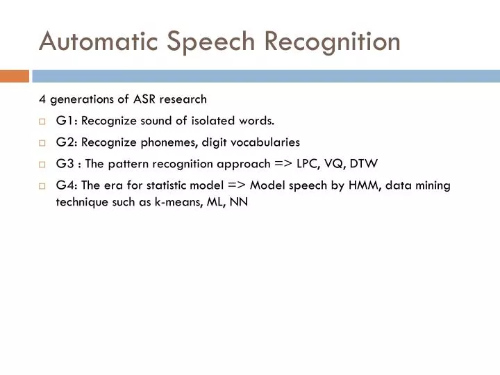
Automatic Speech Recognition. 4 generations of ASR research G1: Recognize sound of isolated words. G2: Recognize phonemes, digit vocabularies G3 : The pattern recognition approach => LPC, VQ, DTW

E N D
Automatic Speech Recognition 4 generations of ASR research • G1: Recognize sound of isolated words. • G2: Recognize phonemes, digit vocabularies • G3 : The pattern recognition approach => LPC, VQ, DTW • G4: The era for statistic model => Model speech by HMM, data mining technique such as k-means, ML, NN
Issue in speech recognition • Speech unit => words, syllable, phoneme • Vocabulary size => small(2-100 words), medium(100-1000), large(>1000 words) • Task syntax => simple syntax, complicated syntax • Speaking mode => isolated words, connected words • Speaker mode => speaker dependent, independent • Speaking situation=>human to machine, human to human • Speaking environment => quiet, noisy • Transducer => phone, cell phone, microphone
Pattern recognition • Dynamic Time warping • Vector Quantization
Dynamic Time Warping (DTW) • An algorithm for measuring similarity between two sequences which may vary in time or speed. • DTW is a method that allows a computer to find an optimal match between two given sequences (e.g. time series) with certain restrictions.
Time Alignment Comparison • Store • Test 1 2 3 4 5 6 1 2 3 4 5 6 7 8 Wrapping path
Time Alignment Comparison • We want to compare two signals A, B • If A is similar to B A B 1 2 3 4 5 6 7 8 1 2 3 4 5 6 7 8 B Time Alignment A 1 1
Time Alignment Comparison • If A is not similar to B A B
Time Alignment Comparison • Time alignment pattern => similarity between two signals • Good match => lowest distortion
Problem • Time Reverse • If we have two signal which are reversed with each other. A B 1 2 3 4 5 6 7 8 1 2 3 4 5 6 7 8 Straight Line not => good match B Time Alignment A 1 1
Time Normalization Constraints The warping path is typically subject to several constraints. • Boundary conditions: w1 = (1,1) and wK = (m,n), simply stated, this requires the warping path to start and finish in diagonally opposite corner cells of the matrix. • Local Continuity: This restricts the allowable steps in the warping path to adjacent cells. • Monotonicity: Temporal order of sequence is an important cue, so avoid a negative slope.
Time Normalization Constraints • Summary of sets of local constraints and the resulting path specifications
Slope Weighting • Slope weighting function m(k) is another dimension of control in the search for the optimal warping path. • There are many slope weighting functions: • Type a • Type b • Type c • Type d
Slope Weighting • Example
Slope Weighting • For type II local continuity 0 1/2 1/2 1 1 1 0 1/2 smooth 1 1/2 • Type a
Optimal path • The overall distortion D(T , S) is based on a sum of local distances between elements d(ti, sj) • D(T , S) =
Vector Quantization • Comparison of the storage rate between raw signal and spectral vector version. Raw signal: sample rate= 10k Hz Amplitude representation = 16-bit So the total storage required is 160,000 bps … 1s coding Spectral vector: vector/second = 100 Amplitude representation = 16-bit Dimension per vector = 10 So the total storage required is 16,000 bps p-dimension V1 V2 V3 V4 V100 10-to-1 reduction
Vector Quantization • Ultimate needing: We want to compress the spectral vector by using only one vector to represent one basic unit such as phoneme. impractical • We can reduce the storage by building a codebook of distinct analysis vector. Vector Quantization
Vector Quantization • VQ is one of the efficient source-coding technique. • VQ is a procedure that encodes a vector of input (segment of waveform, parameter vector) into an integer (index) that is associated with an entry of a collection of reproduction vector (codebook). • The reproduction vector chosen is the one that is closest to the input vector => least distortion.
VQ Procedure • Block diagram of the basic VQ training and classification d(.,.) Clustering Algorithm (k-means) Codebook M=2B vectors Training set of vectors {V1, V2, …,Vl} Quantizer Codebook Indices Input speech vectors d(.,.)
The VQ training Set • The training set vector should span the anticipated range of the following: • Talker: including ranges in age, accent, gender, speaking rate… • Speaking condition: quiet, automobile, noisy… • Transducer, transmission: microphone, telephone… • Speech unit: digit, conversation
Similarity or Distance Measure • The spectral distance measure for comparing spectral vectors vi and vj • Covariance weighted spectral difference • Likelihood • Cepstral distance
Clustering and Training Vectors • The way in which a set of L training vectors can be clustered into a set of M codebook vectors. • K-means clustering algorithm • Initialization: choose M vectors as the initial set of code words in the codebook. • Nearest-Neighbor Search: For each training vector, find the code word in the current codebook that is closest. • Centroid Update: Update the code word centroid • Iteration: repeat step 2 and 3 until the average distance falls below a preset threshold. See the k mean interactive at: http://home.dei.polimi.it/matteucc/Clustering/tutorial_html/AppletKM.html
Vector Classification Procedure • The classification procedure for arbitrary spectral vectors is basically a full search through the codebook to find the “best” match. • We have testing vector v and we want to find the best match code word for v. • Where ymdenote the codebook vectors of an M-vector codebook
Exercise • Find the codebook vector location in the F1-F2 plane for classifying vowels /a/,/e/,/u/ • Each student pronounces vowel /อา//เอ//อู/ 2 times/person • Find F1 and F2 for each vowel • Collect the value of F1 and F2 from other students => data set • Use Weka to cluster these data into 3 clusters.