Download
1 / 16
160 likes | 336 Vues
Molecular phylogenetics 3. Level 3 Molecular Evolution and Bioinformatics Jim Provan. Page and Holmes: Sections 6.5-6. Maximum likelihood. Principle of likelihood suggests that the explanation that makes the observed outcome most probable is preferred More formally: L D = Pr ( D | H )

E N D
Molecular phylogenetics 3 Level 3 Molecular Evolution and Bioinformatics Jim Provan Page and Holmes: Sections 6.5-6
Maximum likelihood • Principle of likelihood suggests that the explanation that makes the observed outcome most probable is preferred • More formally: LD= Pr (D | H) • In a phylogenetic context: • D is the set of sequences being compared • H is a phylogenetic tree • The tree that makes the data the most probable evolutionary outcome is the maximum likelihood estimate of the phylogeny
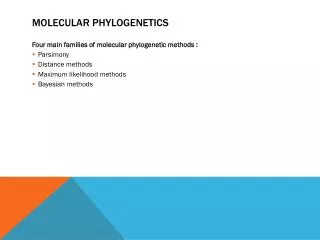
Models, data and hypotheses • Maximum likelihood requires three elements: • A model of sequence evolution • A tree • A data set • ML methods of tree building must solve two problems: • For a given tree topology, what set of branch lengths makes the observed data most likely • Which tree has the greatest likelihood
S k ln L = ln Li i = 1 Models, data and hypotheses • Suppose we have two sequences, 1 and 2, separated by an average of d substitutions per site: d = mt • Given a model of substitution for each site we can compare the probability Pij(d) that two sequences separated by d would have nucleotides i and j: • For example, if sequence 1 had nucleotide A then PAG(d) is the probability that sequence 2 has a G in the corresponding position • The log likelihood of obtaining the observed sequences is the sum of the log likelihoods of each individual site:
-2620 -2640 -2660 -2680 -2700 -2720 -2740 -2760 1 2 3 4 5 6 7 8 9 10 Models, data and hypotheses • What model? • Transition/transversion ratio • Base composition • Variation in rate across sites • In all but simplest models (e.g. Jukes-Cantor), differences in transition / transversion rates can be taken into account • Keeping other parameters constant, it is possible to calculate ML estimates of individual parameters
Likelihood ratio tests • We can test alternative hypotheses concerning the same data using a likelihood ratio test: • Likelihood ratio statistic (D) is the ratio of the alternative hypothesis (H1) to the null hypothesis (H0) • Because likelihoods are often very small, it is more convenient to use log likelihoods: D = log L1 – log L0 where: • L1 is the maximum likelihood of the alternative hypothesis H1 • L0 is the maximum likelihood of the null hypothesis H0 • Can be used to test various hypotheses such as whether a particular model of evolution is valid, whether a molecular clock adequately describes the data or whether one phylogenetic hypothesis is better than another
Observed value 170.70 100 120 140 160 180 Log Lmax – log Ltree Testing models • A model can be tested to measure how well it fits the observed data by comparing likelihood a tree and a model confers on the data (Ltree) with theoretical best (Lmax) • Likelihood ratio test can be performed to test the adequacy of the HKY85 model to describe the hominid mtDNA data set
Clock No clock Gibbon Orang-utan Gorilla Chimp Human Gibbon Orang-utan Gorilla Chimp Human Log L = -2660.61 Log L = -2659.18 Testing rate variation • If sequences are evolving at different rates, then an ultrametric tree will give a poor representation of relationships between taxa: 2D = log Lno clock – log Lclock
S k D = (log L(k, tree 1) - log L(k, tree 2)) = log Ltree 1 - log Ltree 2 i = 1 Human Chimp Gorilla Orang-utan Gibbon Human Chimp Gorilla Orang-utan Gibbon Human Chimp Gorilla Orang-utan Gibbon Log L = -2659.18 Log L = -2663.94 Log L = -2701.36 Comparing phylogenetic hypotheses • If two trees are not significantly different then the sum of these likelihood differences: will not be significantly different from zero
Objections to likelihood • Requires an explicit model of evolution: • This is a strength, since it makes us aware of the assumptions being made • However, dependence on a model raises question of which model to use • Computationally expensive: • Finding the best combination of model and tree is technically difficult • Computing likelihood is also time consuming and it may be that there is more than one maximal likelihood value for a given tree • Suggested that likelihood is better for testing models rather than as an all-purpose phylogenetic tool
Splits • In the above example, the split {{gorilla, orang-utan, gibbon},{human, chimp}} can be written as 00011 in binary notation, or 3 in decimal notation • One advantage is that we can refer to any split by a single number
Spectral analysis • Provides a means of visualising support for each split: • In simple terms, consists of plotting the frequencies of each split in the data set • Straightforward if there is two states for each character Human G T C A T C A T C C 1 1 0 1 1 0 1 1 0 1 Chimp A T T A C C A T T C 0 1 1 1 0 0 1 1 1 1 Gorilla G T T G T T A T T A 1 1 1 0 1 1 1 1 1 0 Orang-utan A C C A C T C C C A 0 0 0 1 0 1 0 0 0 0 Gibbon A C C G C C C C C A 0 0 0 0 0 0 0 0 0 0 5 7 6 11 5 12 7 7 6 3
0.05 0.04 0.03 0.02 0.01 0.00 H C H C Go H Go C Go O Gi O H O C O Go Gi Go O C Gi H Gi Gi Spectral analysis
Spectral analysis • Since all splits cannot coexist in the same tree, some method is needed to decide which splits to use to construct the tree: • Five “trivial” splits will be in every tree • One possible solution is to choose the two mutually compatible, non-trivial splits which have the best support: • In this case, the best non-trivial split is {Orang-utan, Gibbon} • The next best supported split is {Human, Chimp}, which is compatible with this split • This gives the basic topology {{Human, Chimp}, Gorilla, {Orang-utan, Gibbon}} • Problems with spectral analysis: • Computationally expensive (half a million splits for 20 sequences) • Potential for more than two character states
H 1 O B 1 H O B H C O C G 2 G B C G Split decomposition 1 2 3 4 5 6 7 8 9 HumanT C C T T A A A A ChimpT T C T A T A A A GorillaT T A C A A T A A Orang-utanC C A C A A A T A GibbonC C A C A A A A T
3 4 1 O B 3 1 H O B H 2 2 2 2 C G C G 3 3 4 3 3 H O 5 8 3 4 1 2 2 9 B 6 7 3 3 4 C G Split decomposition