Download
1 / 48
490 likes | 655 Vues
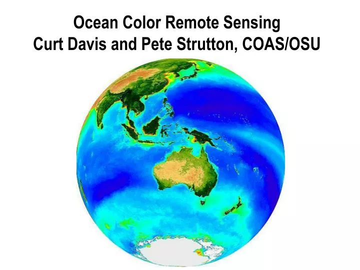
Ocean Color Remote Sensing Curt Davis and Pete Strutton, COAS/OSU. Presentation Outline. What do we mean by ‘Ocean Color’? How are the measurements made? What parameters can be derived? What are these data used for? Where are the data available?. Components of a remote sensing system.

E N D
Ocean Color Remote Sensing Curt Davis and Pete Strutton, COAS/OSU
Presentation Outline • What do we mean by ‘Ocean Color’? • How are the measurements made? • What parameters can be derived? • What are these data used for? • Where are the data available?
Components of a remote sensing system sensor source raw data signal processing / dissemination cal/val
Ocean color (chlorophyll) • Passive measurement - energy source is the Sun • In contrast to altimetry, SST etc, looks at subsurface, not ‘skin’ • Measures light emitted from the ocean (careful to distinguish between ‘emission’ and ‘reflection’) • Actual parameter measured (raw data) is the total radiance at the sensor Lt • Most of the signal (>90%) at the satellite is reflected by the atmosphere and the sea surface – atmospheric correction is performed to remove these signals and obtain the desired signal normalized water leaving radiance, (nLw ) or remote sensing reflectance Rrs • Also interference from other colored material in the ocean, e.g. sediments, ‘colored dissolved organic matter’ (CDOM).
u NADP + 2H+ NADPH2 2 e- LHC ADP+P ATP Fluorescence ff heat fh Focus on Chlorophyll / Ocean Photosynthesis
The ocean color measurement and how it’s used Main signals: Atmosphere,reflection from the sea surface and ocean color Lt Ed Lw
Measuring chlorophyll from space The Sea-viewing Wide Field of view Sensor: SeaWiFS The satellite The instrument
What SeaWiFS sees in one day The gap here is caused by the satellite tilting as it passes over the equator
Clouds and other challenges Clouds • Severity varies with location and season • When viewing multi-day composites, variable ‘sample size’ • Coastal fog can have the same effect as clouds Other complicating factors • Atmospheric aerosols • Colored dissolved organic matter (CDOM) - mostly breakdown products from phytoplankton and terrestrial sources. • Other components of river runoff such as sediments. • Diminished in open ocean, aka Case I waters
Chlorophyll fluorescence Light energy not used for photosynthesis is lost as heat and fluorescence Fp +Ff + Fh = 1 u NADP + 2H+ NADPH2 2 e- LHC ADP+P ATP Fluorescence ff heat fh
Blue light induced chlorophyll fluorescence in Tobacco leaf. A. photographed in white light. B. taken in the low steady state of fluorescence, 5 min after the onset of illumination. The bright red fluorescing upper part of the leaf is where photosynthesis has been blocked by the herbicide duiron (DCMU). (From Krause and Weis, 1988) u e- PSI LHC (ATP & NADPH2) L683 heat u DCMU PSI LHC (ATP & NADPH2) L683 heat Fp + Ff + Fh = 1
FLH vs. chlorophyll FLH vs. CDOM
MODIS Terra L2 1 km resolution scene from October 3rd 2001 Sea Surface Temperature Chl a Chl Fluorescence Line Height (°C) (mg m-3) (W m-2 mm-1 sr-1) From OSU-COAS EOS DB Station
Chlorophyll fluorescence from space • Passive measurement (sun is the initial source) • Offers the possibility of phytoplankton physiology from space • Also potentially a chlorophyll proxy that is unaffected by: • Sediments • Other colored material • However, signal is very small, and our understanding is evolving
Satellite-based productivity algorithms Motivation: Chlorophyll measurements give biomass, we want productivity (rate) Global coverage 1000s of 14C measurements of primary productivity have been made and continue to be made Do not accurately reflect global temporal and spatial variability Need models of primary productivity - take satellite data as input and provide integrated primary productivity as the output Allows us to quantify the spatial distribution of productivity, but also… Temporal changes at time scales from days to decades (NASA's main goal)
Other Ocean Color Products Particulate Organic Carbon (POC): Potentially more useful for carbon budgets than phytoplankton chlorophyll Particulate Inorganic Carbon (PIC): Indicative of a specific type of phytoplankton (coccolithophorids), common in polar waters. Photosynthetically Available Radiation (PAR) Diffuse attenuation coefficient Terrestrial biosphere products
The sensors and data SeaWiFS: Launched 1997, very successful, well-calibrated and still operating? MODIS Aqua: Launched 2002, has fluorescence channel that SeaWiFS lacks. Data available at spatial resolutions from ~1km to 9km Data available at daily resolution with the caveats previously discussed Data gateway depends on user: NASA directly, CoastWatch, others…
The need for High Spatial Resolution in the Near Coastal Ocean SeaWiFS 1 km data PHILLS-2 9 m data mosaic Near-simultaneous data from 5 ships, two moorings, three Aircraft and two satellites collected to address issues of scaling in the coastal zone. (HyCODE LEO-15 Experiment July 31, 2001.) Sand waves in PHILLS-1 1.8 m data Fronts in AVIRIS 20 m data
Resolving the Complexity of Coastal OpticsRequires Imaging Spectrometry Extensive studies using shipboard measurements and airborne hyperspectral imaging have shown that visible hyperspectral imaging is the only tool available to resolve the complexity of the coastal ocean from space. (Lee and Carder, Appl. Opt., 41(12), 2191 – 2201, 2002.)
Solving the Shallow Ocean Remote Sensing Problem using Hyperspectral Data Remote-sensing reflectance (Rrs = Lu/Ed at the sea surface) is a function of properties of the water column and the bottom, Rrs() = f[a(), bb(), (), H],(1) where a() is the absorption coefficient, bb() is the backscattering coefficient, () is the bottom albedo, H is the bottom depth. Wherea() is the sum of awater + aphytoplankton + aCDOM + Detritus And bb()is the sum of bb water + bb phytoplankton + bb detritus + bb sediments It is desired to simultaneously derive bottom depth and albedo and the optical properties of the water column. This is done by taking advantage of the spectral characteristics of the absorption and reflectance characteristics of the water column constituents and the bottom. The next three slides show examples of how bottom albedo, water optical properties and depth effect remote sensing reflectance:
AN-2 Aircraft PHILLS Sensor The NRL Portable Hyperspectral Imager for Low-light Spectroscopy (PHILLS) PHILLS image of shallow water features near Lee Stocking Island, Bahamas used to develop and validate hyperspectral algorithms for bathymetry, bottom type and water clarity. Ocean PHILLS is a push-broom imager. f 1.4 high quality lens, color corrected and AR coated for 380 –1000nm. all reflective spectrograph with a convex grating in an Offner configuration to produce a distortion free image (Headwall, Fitchburg, MA ). 1024 x 1024 thinned backside illuminated CCD camera (Pixel Vision, Inc, Beaverton, OR). Images 1000 pixels cross track and is typically flown at 3000 m altitude yielding 1.5 m GSD and a 1500 m wide sample swath. (C. O. Davis, et al., (2002), Optics Express 10:4, 210--221.)
Bathymetry, Bottom Type and Optical Properties using Look-up Tables Interpretation of hyperspectral remote-sensing imagery via spectrum matching and look-up tables, Mobley, C. D., et al., 2005, Applied Optics, 44(17):3576-3592.
Bloom disappears on the 15th 9:11 9:34 Sept 15, 2006: No bloom images by Maria Kavanaugh
Rrs [sr-1] St.11 St.10 St.10 Rrs [sr-1] Wavelength [nm] [Chl] was ~ 500 mg/m3. St.11 MERIS remote sensing reflectance (Rrs) compared with in situ measurements Monterey Bay (CA), Sept. 11, 2006 Data from Z.-P. Lee, NRLSSC
Atmospheric Correction for Turbid Waters in Coastal Regions: Menghua Wang NOAA/NESDIS/ORA E/RA3, Room 102, 5200 Auth Rd. Camp Springs, MD 20746, USA Menghua.Wang@noaa.gov The Coastal Ocean Applications and Science Team Meeting September 7-8, 2005, Corvallis, Oregon
Solar Irradiance Passive Remote Sensing: Sensor-measured signals are all originated from the sun!
Ocean Color Remote Sensing Sensor-Measured “Green” ocean Blue ocean Atmospheric Correction (removing >90% signals) Calibration (0.5% error in TOA >>>> 5% in surface) From H. Gordon
Atmospheric Windows UV bandscan be used for detecting the absorbing aerosol cases Two long NIR bands (1000 & 1240 nm)are useful for of the Case-2 waters
The Ocean Radiance Spectrum TOA Reflectance Open Ocean Waters Coastal Waters
Atmospheric Correction MODISand SeaWiFS algorithm (Gordon and Wang 1994) • wis thedesired quantity in ocean color remote sensing. • Tgis the sun glint contribution—avoided/masked/corrected. • Twcis the whitecap reflectance—computed from wind speed. • risthe scattering from molecules—computed using the Rayleigh lookup tables (atmospheric pressure dependence). • A = a+rais the aerosol and Rayleigh-aerosol contributions —estimated using aerosol models. • For Case-1 waters at the open ocean,wis usually negligibleat750 & 865 nm. A can be estimated using these two NIR bands. Ocean is usually not black at NIR for the coastal regions. Gordon, H. R. and M. Wang, “Retrieval of water-leaving radiance and aerosol optical thickness over the oceans with SeaWiFS: A preliminary algorithm,” Appl. Opt., 33, 443-452, 1994.
SeaWiFS Chlorophyll-a Concentration(October 1997-December 2003)