Download
1 / 84
870 likes | 1.3k Vues
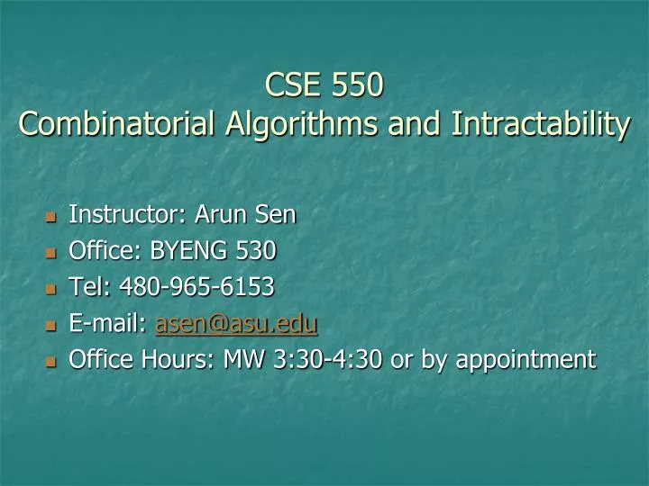
CSE 550 Combinatorial Algorithms and Intractability. Instructor: Arun Sen Office: BYENG 530 Tel: 480-965-6153 E-mail: asen@asu.edu Office Hours: MW 3:30-4:30 or by appointment. Two additional (recommended) books. Approximation Algorithms for NP-hard Problems – Dorit S. Hochbaum

E N D
CSE 550Combinatorial Algorithms and Intractability • Instructor: Arun Sen • Office: BYENG 530 • Tel: 480-965-6153 • E-mail: asen@asu.edu • Office Hours: MW 3:30-4:30 or by appointment
Two additional (recommended) books • Approximation Algorithms for NP-hard Problems – Dorit S. Hochbaum • Approximation Algorithms – Vijay V. Vazirani
Grading Policy • There will be one mid-term and a final. In addition, there will be programming and homework assignments • Mid-term 30% • Final 40% • Assignments 30% • For 90% will ensure A, 80% will ensure B, 70% will ensure C and so on • Loss of points due to late submission of assignments • 1 day 50% • 2 days 75% • 3 days 100%
What is a Combinatorial Algorithm? • A combinatorial algorithm is an algorithm for a combinatorial problem. • What is a Combinatorial Problem? • Combinatorics is the branch of mathematics concerned with the study of arrangements, patterns, designs, assignments, schedules, connections and configurations. • Examples • A shop supervisor prepares assignments of workers to tools or work areas • An Industrial Engineer considers production schedules and workplace configurations to maximize production • A geneticist considers arrangements of bases into chains of DNA and RNA
Types of Combinatorial Problems • Three types of problems in Combinatorics • Existence Problems • Counting Problems • Optimization Problems • Optimization Problems are concerned with the choice of the “best” (according to some criterion) solution among all possible solutions. • In this class, we will focus on optimization and related problems.
How many binary trees can you draw with n nodes? n=1: b1=1 n=2: b2=2 n=3: b3=5
How many binary trees can you draw with n nodes?Suppose b(n) is the number of binary trees that can be constructed with n nodes. In that case, b(n) can be expressed with the following recurrence relation
Combinatorial Problem in Manufacturing Various wafers (tasks) are to be processed in a series of stations. The processing time of the wafers in different stations is different. Once a wafer is processed on a station it needs to be processed on the next station immediately, i.e., there cannot be any wait. In what order should the wafers be supplied to the assembly line so that the completion time of processing of all wafers is minimized?
w1 t11 t12 t18 S1 S2 S8 w2 t21 t22 t28 w3 t31 t32 t38
w1 : t11 = 4, t12= 5; w2 : t21 = 2, t22 = 4; w1 : w2 : w2: w2 : w1: Completion Time in the first ordering = 13 Completion Time in the second ordering = 11
Sensor Placement Problem Sensor Placement in a Temperature Sensitive Environment
Sensor Placement Problem Sensor Placement in a Temperature Sensitive Environment
Sensor Placement Problem • Bio-sensors implanted in human body dissipate energy during their operation and consequently raise the temperature of the surrounding. • A temperature sensitive environment like the human body or brain can tolerate increase in temperature only up to a certain threshold. • One needs to make sure that the rise in temperature due to the operation of implanted bio-sensors in temperature sensitive environments such as human/animal body does not exceed the threshold and cause any adverse impact.
Thermal Model and Analysis • A sensor is expected to operate for a certain duration of time. • The rise is temperature in the area surrounding the sensor will be dependent on the duration of operation. • The sensor surroundings will attain a maximum temperature during the time of operation (steady state temperature). • If the steady state temperature of a sensor exceeds the maximum allowable threshold in the surrounding, such a sensor cannot be deployed. • Question: Is it possible that a sensor whose steady state temperature does not exceed the threshold when operating in isolation, may exceed the threshold when operating with multiple other sensors?
Thermal Model and Analysis • We perform a thorough analysis of the heat distribution phenomenon in a temperature sensitive environment and come to the following conclusion: There exists a critical inter-sensor distance dcr, such that if the distance between any two deployed sensors is less than dcr, then the temperature in the vicinity of the sensors will exceed the maximum allowable threshold. Therefore, attention must be paid during sensor deployment to ensure that the distance between any two sensors is at least as large as dcr.
Sensor Coverage Problem • Given: • A set of locations (or points pi) to be sensed • A set of potential locations (or points q i ) for the placement of the sensors • A minimum separation distance (dcr) between each pair of sensors. • Objective: • To deploy as few sensors as possible in the potential placement locations such that all points pi are sensed and the distance between any two sensors is at least as large as dcr. • Assumption • Each sensor is capable of sensing a circular area of radius rsen with the location of the sensor being the center of the circle.
Sensor Coverage Problem • Formal definition:
Search Space • The solution is somewhere here • Solution can be found by exhaustive search in the search space • Search space for the solution may be very large • Large search space implies long computation time to find solution (?) • Not necessarily true • Search space for the sorting problem is very large • The trick in the design of efficient algorithms lies in finding ways to reduce the search space
Evaluating Quality of Algorithms • Often there are several different ways to solve a problem, i.e., there are several different algorithms to solve a problem • What is the “best” way to solve a problem? • What is the “best” algorithm? • How do you measure the “goodness” of an algorithm? • What metric(s) should be used to measure the “goodness” of an algorithm? • Time • Space ** What about Power?
Problem and Instance • Algorithms are designed to solve problems • What is a problem? • A problem is a general question to be answered, usually processing several parameters, or free variables, whose values are left unspecified. A problem is described by giving (i) a general description of all its parameters and (ii) a statement of what properties the answer, or the solution, required to satisfy. • What is an instance? • An instance of a problem is obtained by specifying particular values for all the problem parameters.
Traveling Salesman Problem Instance: A finite set C={c1, c2, …, cm} of cities, a distance d(ci, cj) є Z+ for each pair of cities ci, cj є C and a bound B є Z+ (where Z+ denotes the positive integers). Question: Is there a tour of all cities in C having total length no more than B, that is an ordering <cπ(1), cπ(2), …, cπ(m)> of C such that,
Algorithms are general step-by-step procedures for solving problems. • An algorithm is said to solve a problem Πif that algorithm can be applied to any instance I of Πand is guaranteed always to produce a solution for that instance I. • In general we are interested in finding the most efficient algorithm for solving a problem. • The time requirements of an algorithm are expressed in terms of a single variable, the size of a problem instance, which is intended to reflect the amount of input data needed to describe the instance.
Measuring efficiency of algorithms • One possible way to measure efficiency may be to note the execution time on some machine • Suppose that the problem P can be solved by two different algorithms A1 and A2. • Algorithms A1 and A2 were coded and using a data set D, the programs were executed on some machine M • A1 and A2 took 10 and 15 seconds to run to completion • Can we now say that A1 is more efficient that A2?
Measuring efficiency of algorithms • What happens if instead of data set D we use a different dataset D’? • A1 may end up taking more time than A2 • What happens if instead of machine M we use a different machine M’? • A1 may end up taking more time than A2 • If one want to make a statement about the efficiency of two algorithms based on timing values, it should read “A1 is more efficient that A2 on machine M, using data set D”, instead of an unqualified statement like “A1 is more efficient that A2”
Measuring efficiency of algorithms • The qualified statement “A1 is more efficient that A2 on machine M, using data set D” is of limited value as someone may use different data set or a different machine • Ideally, one would like to make an unqualified statement like “A1 is more efficient that A2” , that is independent of data set and machine • We cannot make such an unqualified statement by observing execution time on a machine • Data and Machine independent statement can be made if we note the number of “basic operations” needed by the algorithms • The “basic” or “elementary” operations are operations of the form addition, multiplication, comparison etc
Analysis of Algorithms .00002 sec .00003 sec .00004 sec .00005 sec .00006 sec .0001 sec .0004 sec .0009 sec .0016 sec .0025 sec .0036 sec .001 sec .008 .027 .064 .125 .216 sec sec sec sec sec .1 sec 3.2 sec 24.3 sec 1.7 min 5.2 min 13.0 min .001 sec 1.0 sec 17.9 min 12.7 days 35.7 years 366 centuries .059 sec 58 6.5 3855 2*108 1.3*1013 min years cents. cents. cents.
Size of Largest Problem Instance Solvable in 1 Hour 100 N1 1000 N1 10 N2 31.6 N2 4.64 N3 10 N3 2.5 N4 3.98 N4 N5 + 6.64 N5 + 9.97 N6 + 4.19 N6 + 6.29
Growth of Functions: Asymptotic Notations O(g(n)) = {f(n): there exists positive constants c and n0such that 0<=f(n)<=c * g(n) for all n >= n0} Ω(g(n)) = {f(n): there exists positive constants c and n0 such that 0<=c * g(n)<=f(n) for all n >= n0} Q(g(n)) = {f(n): there exists positive constants c1, c2 and n0 such that 0<= c1 * g(n)<=f(n)<=c2*g(n) for all n >= n0} o(g(n) = {f(n): for any positive constant c>0 there exists a constant n0>0 such that 0<=f(n)<c * g(n) for all n >= n0} w(g(n)) = {f(n): for any positive constant c>0 there exists a constant n0 such that 0<=<c * g(n)< f(n) for all n >= n0} A function f(n) is said to be of the order of another function g(n) and is denoted by O(g(n)) if there exists positive constants c and n0such that 0<=f(n)<=c * g(n) for all n >= n0}
Basic Operations and Data Set • To evaluate efficiency of an algorithm, we decided to count the number of basic operations performed by the algorithm • This is usually expressed as a function of the input data size • The number of basic operations in an algorithm • Is it independent of the data set ? • Is it dependent on the data set?
Given a set of records R1, …, Rn with keys k1, …,kn. Sort the records in ascending order of the keys.
Basic Operations and Data Set • The number of basic operations in an algorithm • Is it independent of the data set ? • Is it dependent on the data set? • If the number of basic operations in an algorithm depends on the data set then one needs to consider • Best case complexity • Worst case complexity • Average case complexity • What does “average” mean? • Average over what?
Given n elements X[1], …, X[n], the algorithm finds m and j such that m = X[j] = max 1<=k<=n X[k], and for which j is as large as possible. Algorithm FindMax Step 1. Set j n, k n – 1, m X[n] Step 2. If k=0, the algorithm terminates. Step 3. If X[k] <= m, go to step 5. Step 4. Set j k, m X[k]. Step 5. Decrease k by 1, and return to step 2
Computational Speed-up and the Role of Algorithms • Moore’s law says that computing power (hardware speed) doubles every eighteen months • How long will it take to have a thousand-fold speed-up in computation, if we rely on hardware speed alone? • Answer: 15 years • Expected cost: significant • How long will it take to have a thousand-fold speed-up in computation, if we rely on the design of clever algorithms? • Thousand-fold speed-up can be attained if currently used O(n5) complexity algorithm is replaced by a new algorithm with complexity O(n2) for n=10. • How long will it take to develop a O(n2) complexity algorithm which does the same thing as the currently used O(n5) complexity algorithm? • Answer: May be as little as one afternoon • Ingredients needed • Pencil • Paper • A beautiful mind • Expected cost: significantly less than what will be needed if we rely on hardware alone
Computational Speed-up and the Role of Algorithms • A clever algorithm can achieve overnight what progress in hardware would require decades to accomplish. • “The algorithm things are really startling, because when you get those right you can jump three orders of magnitude in one afternoon.” William Pulleyblank Senior Scientist, IBM Research
Algorithm Design Techniques • Divide and Conquer • Dynamic Programming • Greedy Algorithms • Backtracking • Branch and Bound • Approximation Algorithms • Probabilistic (Randomized) Algorithms • Mathematical Programming • Parallel and Distributed Algorithms • Simulated Annealing • Genetic Algorithms • Tabu Search
How do you “prove” a problem to be “difficult”? • Suppose that the algorithm you developed for the problem to be solved (after many sleepless nights) turned out to be very time consuming • Possibilities • You haven’t designed an efficient algorithm for the problem • May be you are not that great an algorithm designer • May be you are a better fashion designer • May be you have not taken CSE 450/598 • May be the problem is difficult and more efficient algorithm cannot be designed • How do you know that more efficient algorithm cannot be designed? • It is difficult to substantiate a claim that more efficient algorithm cannot be designed • Your inability to design an efficient algorithm does not necessarily mean that the problem is “difficult” • It may be easier to claim that the problem “probably” is “difficult” • How do you substantiate the claim that the problem “probably” is “difficult”? • What if you line up a bunch of “smart” people who will testify that they also think that the problem is difficult? • Theory of NP-Completeness
Problems Taxonomy of Problems Undecidable Decidable Intractable (deterministically) Tractable (deterministically) Tractable (non-deterministically) Intractable (non-deterministically) NP-Complete Problems (Most likely deterministically Intractable
Complexity of Algorithms and Problems • In algorithms classes (e.g., CSE 450) we make distinctions between algorithms of complexity O(n2), O(n3), and O(n5). • In this class, we take a much coarse grain view and divide algorithms into only two classes – polynomial time algorithms and non-polynomial time algorithms. • Polynomial time algorithms – Good • Non-polynomial time algorithms - Bad
Good vs. Bad (in Algorithms) • Exponential time algorithms should not be considered “good” algorithms. • Most exponential time algorithms are merely variations of exhaustive search. • Polynomial time algorithms generally are made possible only through gain of some deeper insight into the structure of a problem.
Easy and Difficult Problems • A problem is easy if a polynomialtime algorithm is known for it. • A problem may be suspected to be difficult if a polynomialtime algorithm cannot be developed for it, even after significant time and effort.
Theory of NP-Completeness • Complexity of an algorithm for a problem says more about the algorithm and less about the problem • If a low complexity algorithm can be found for the solution of a problem, we can say that the problem is not difficult • If we are unable to find a low complexity algorithm for the solution of a problem, can we say that the problem is difficult? • Answer: No • NP-Completeness of a problem says something about the problem • Problems may or may not be NP-Complete – not the algorithms
Problems and Algorithms for their solution Problem P Algorithm 3 Complexity: O(2n) Algorithm 1 Complexity: O(n) Algorithm 2 Complexity: O(n4)