Download
1 / 18
180 likes | 314 Vues
Using combined Lagrangian and Eulerian modeling approaches to improve particulate matter estimations in the Eastern US. Ariel F. Stein 1 , Rohit Mathur 2 , Daiwen Kang 3 and Roland R. Draxler 4 1 Earth Resources & Technology (ERT) on assignment to the Air Resources Laboratory (ARL) at NOAA

E N D
Using combined Lagrangian and Eulerian modeling approaches to improve particulate matter estimations in the Eastern US. Ariel F. Stein1, Rohit Mathur2, Daiwen Kang3 and Roland R. Draxler4 1Earth Resources & Technology (ERT) on assignment to the Air Resources Laboratory (ARL) at NOAA 2Atmospheric Science Modeling Division (ASMD), ARL-NOAA 3 Science and Technology Corporation on assignment to ASMD/ARL 4Air Resources Laboratory (ARL) at NOAA
Motivation • Underestimations in PM: CMAQ domain is not big enough toinclude long range transport. • Example: Forest fires in Alaska. July 14th to 23rd of 2004. • Summer 2004: One of the strongest fire seasons on record for Alaska and Western Canada • Smoke plume from Alaska transported into continental US • PM2.5 grossly under-predicted by ETA-CMAQ forecast system • Model picks up spatial signatures ahead of the front • Simulation under predicts behind the front
Forest fires emissions HYSPLIT HYSPLIT-CMAQ interface CMAQ System description
Emissions • Fire locations from Hazard Mapping System Fire and Smoke Product (http://www.ssd.noaa.gov/PS/FIRE/hms.html) • The fire position data representing individual pixel hot-spots that correspond to visible smoke are aggregated on a 20 km resolution grid. • Each fire location pixel is assumed to represent one km2 and 10% of that area is assumed to be burning at any one time. • PM2.5 emission rate is estimated from the USFS Blue Sky (http://www.airfire.org/bluesky) emission algorithm, which includes a fuel type data base and consumption and emissions models
The smoke outlines are produced manually, primarily utilizing animated visible band satellite imagery. The locations of fires that are producing smoke emissions that can be detected in the satellite imagery are incorporated into a special HMS file that only denotes fires that are producing smoke emissions. These fire locations are used as input to the HYSPLIT model. HMS map for July 13th 2004
HYSPLIT • Same settings as in the Interim Smoke Forecast Tool • Mass distribution: • Horizontal: Top hat • Vertical: 3D Particle • Number of lagrangian particles per hour: 500 • Release height: 100 m • Meteorology: NCEP Global Data Assimilation System (GDAS, horizontal resolution 1x1 deg) • Run as in forecast mode: Each calculation is started with all the pollutant particles that are on the domain at the model's initialization time as computed from the previous day's simulation (yesterday's 24 h forecast). • Smoke particles are assumed to have a diameter of 0.8 mm with a density of 2 g/cc • Wet removal is much more effective than dry deposition and smoke particles in grid cells that have reported precipitation may deposit as much as 90% of their mass within a few hours
Advection and Dispersion • P(t+Dt) = P(t) + 0.5 [V(P,t) + V(P’,t+Dt)] Dth • P’(t+Dt) = P(t) + V(P,t) Dth • Umax(grid units min-1) Dth(min) < 0.5 (grid units) • Xfinal(t+Dt) = Xmean(t+Dt) + U’(t+Dt) Dt • Zfinal(t+Dt) = Zmean(t+Dt) + W’(t+Dt) Dt
HYSPLIT-CMAQ preprocessor • This processor reads the location of each lagrangian particle as calculated by HYSPLIT and determines the concentration of the pollutant at the boundaries of the CMAQ domain. • The concentration of each chemical species within a boundary cell is calculated by: • In the vertical: dividing the sum of the particle masses of a particular chemical compound by the height of the corresponding concentration grid cell in which the particles reside • In the horizontal: the concentration grid is considered as a matrix of sampling points, such that the puff only contributes to the concentration as it passes over the sampling point C = q ( pr2 zp)-1 • A speciation profile was applied to obtain the chemical species compatible with CMAQ’s chemical mechanism. It was assumed that the composition of PM2.5 was 77% organic carbon , 16% elemental carbon, 2% sulfate, 0.2% nitrate and 4.8% other PM.
CMAQ v4.5 • 259 Columns x 268 Rows • 12x12 km horizontal resolution covering Eastern US • 22 Vertical layers • Meteorology driven by ETA • Emissions: SMOKE • Chemistry: EBI CB4 • Aerosols: Isorropia AERO3 • Advection: YAMO New global mass-conserving scheme (Robert Yamartino) • Clouds: Asymmetrical Convective Model (ACM)
7/17 7/18 7/19 MODISAOD 0 0.1 0.2 0.3 0.4 0.5 0.6 0.7 0 0.1 0.2 0.3 0.4 0.5 0.6 0.7 CMAQ NO BC AOD DIFF HYSPLIT-CMAQ to CMAQ AOD 0 0.004 0.015 0.026
AOD under estimation • Transport and dispersion? Not likely. Timing and geographical extension of smoke plume is very good compared with satellite images • Dry deposition? Not likely. Sensitivity shows no substantial variation in output. • Emission’s initial height? No. Sensitivity run with 2000m release height shows no substantial difference with base case. • Emission’s strength? Very uncertain. Could be off by a factor of 10.
Emissions sensitivity Emissions scaled to daily total Pfister’s emissions Emissions x 10 Pfister, G, Hess P.G., Emmons L.K., Lamarque J.-F., Wiedinmyer C., Edwards D.P., Petron G., Gille J.C., and Sachse G.W., 2005. Quantifying CO emissions from 2004 Alaskan wildfires using MOPITT CO data. Geophysical Research Letters, Vol. 32, L11809.
LIDAR vs CMAQ at Madison WI July 19th 0 UTC July 19th 12 UTC July 18th 12 UTC PBL height PBL height PBL height
Conclusions and future activities • Coupled models capture the main features of PM long range transport • Magnitude of PM emissions are an issue • Advantage of using HYSPLIT: vertical distribution of PM • Integrate operational HYSPLIT interim forecast system with operational CMAQ forecast system? • How about dust?