Download
1 / 39
410 likes | 581 Vues
MRI preprocessing and segmentation. Bias References. Segmentation References. Validation. Segmentation pipeline. Clarke, 1995. 1. Preprocessing 1.1. Brain extraction 1.2. Removal of field inhomogeneities (bias-field). 1.1. Brain extraction.

E N D
MRI preprocessing and segmentation
Validation Segmentation pipeline Clarke, 1995
1. Preprocessing 1.1. Brain extraction 1.2. Removal of field inhomogeneities (bias-field)
1.1. Brain extraction MRI of head Intracranial volume Extracted brain
1.1. Brain extraction FSL: Initiate a mesh inside the skull and expand-wrap onto brain surface Huh, 2002 method: go to mid sagittal, find brain, copy mask on adjacent slices correct the copied mask
1.1. Brain extraction initial mask adjacent slice j mask of slice j Huh, 2002 challenge
1.1. Brain extraction restoring truncated boundary
Let voxel have a value 1 if its intensity is higher than t (determine t arbitrarily, increase when needed)
S I 20 % 1.2. Removal of field inhomogeneities Bias field Phantom studies: Typical signal falloff in SI direction is 20% intensity x
1.2. Removal of field inhomogeneities Statistical methods: probabilistic, gaussian and mixture models of bias-field Polynomial methods: smooth polynomial fit to bias-field
1.2. Removal of field inhomogeneities Polynomial method example: Milchenko, 2006
orig model bias result 1.2. Removal of field inhomogeneities Shattuck, 2001
2. Feature extraction Features: - Intensities in a single MRI: univariate classification - Feature vector from a single MRI: multi-variate class. ex: [I(x,y,z) f(N(x,y,z)) g(N(x,y,z))] where N : neighbourhood around (x,y,z) f: distribution of I in neighborhood (entropy) g: average I in neighborhood or f, g specify edge or boundary information - Intensities in multiple MRIs with different contrast: multi-variate (multi-spectral)
3. Segmentation 3 tissue types: CSF, GM, WM 4 regions: R1: air, scalp, fat, skull (background, removed) R2: subarachnoid space (CSF) R3: parenchyma (GM, WM) R4: ventricles(CSF)
3. Segmentation (dual echo:T2, PD or T1, T2, PD weighted) (T1 weighted) Clarke, 1995
3. Segmentation T1 weighted, single intensity dual echo:T2, PD or T1, T2, PD weighted or T1 weighted with feature vector 3.1. Histogram based thresholding 3.2. Bayesian Unsupervised 3.6. k-means 3.7. fuzzy cmeans Supervised Parametric Non-parametric ANN 3.3. Max. Likelihood 3.4. k-NN 3.5. MLP
3.1. Histogram based thresholding WM GM Lcp crossing point of tangents Histogram of extracted, bias corrected brain in T1-weighted MRI L = g * Lcp (set g manually on 80 images) if I(x,y,z) < L then GM else WM Schnack, 2001
Population1 Population2 Population3 3.2. Bayesian segmentation GM WM (#of voxels/#ofallvoxels in the brain) (intensity) Hypothetical distributions
3.2. Bayes’ classifier For each voxel, x,y,z: Assume K tissue types (for eg. T1, T2, ..., Tk) possible, for 1 observed intensity, I: setup graphs above from regional data GM, WM, CSF ratios from volumetric studies P(Tj ! I) = P(I ! Tj) . P(Tj) Ξ P(I ! Tk). P(Tk) k J,k=1,2,3: 1: CSF, 2: GM, 3:WM Decide on tissue type m if: P(Tm ! I) > P(Tj ! I) for all j Kovacevic, 2002
Methods based on feature vector or multi-spectral data Supervised vs unsupervised Methods Supervised: - Color indicates known classes - Separation contour is to be found during training phase - Separation contour is used for classification during recall phase Unsupervised: - No color, classes unknown - Clusters are found during training phase - Association with clusters are made during recall phase
PD weighted image intensity intensity voxel x,y,z T2 weighted T2 weighted image Kovacevic, 2001
3.3. Maximum likelihood classifier - Assume the distribution P(I ! Tj) in Bayes can be obtained by a mixture of Gaussian or Normal distribution - Estimate means and co-variance matrix - For better results use Hidden Markov fields within neighborhoods 15 classes Zavaljevski, 2000
3.3. Maximum likelihood classifier Zavaljevski, 2000 Normal subject Stroke patient
3.4. K-NN, K-Nearest neighbor classifier Hypothetical distribution T2 intensity T1 intensity - k is always odd, 1<k<15 (as k increases comput time increases) - given a point p find k closest samples known from before - decide on class m where m is the highest number of classes among these k samples
3.4. K-NN classifier Uses 5 different contrast MRIs manual atlas labels atlas labels labels with linear reg. with non-lin reg. k=1 k=45 Vrooman, 2007
3.5. ANN, MLP classifier for segmentation, M = 3, 3 classes :F MLP Architecture: 1 layer: linear contour >1 layers: complex contours countours are used for class separation W1 W3 feature vector transfer fcn: sigmoid
3.5. ANN, MLP classifier Results This page is empty on purpose
3.6. k-means classifier This classifier is not used much in segmentation, but explained here as an introduction to fuzzy c-means Algorithm: - k is equal to number of classes - choose k arbitrary initial seed points (*) - assume seed points are class centroids 1 for each sample point j, find distance to all k centroids Let j belong to class m if j is closest to centroid m 2 for each class k, recalculate centroids repeat steps 1 and 2 above until no change in centroids Note how class assignments change at each iteration Minimized measure:
3.7. fuzzy c-means (FCM) classifier k-means classifier FCM classifier U: membership row=each sample x col=each class minimized cost
If || U(k+1) - U(k)||< 3.7. fuzzy c-means (FCM) classifier Initialize U=[uij] matrix, U(0) At k-step: calculate the centers vectors C(k)=[cj] with U(k) initial iteration 8 iteration 37 Update U(k) , U(k+1)
3.7. fuzzy c-means classifier Results
4. Validation Important issues: - Partial volume effect, visualization - Validation in manually segmented image - Performance comparison with other methods on simulated image: Ex: Brainweb from Mcgill
4. Validation Clark, 2006 Partial volume effect for boundary separation Shattuck, 2001 segmented gold std corrrect WM misclassified (colored by subejct number there are a total of 10 subjects)