Download

1 / 12
120 likes | 202 Vues
Drawing with Precision. Lesson 2. Now that you can draw objects……. Let’s create them to a specific size and location. 4” DIA. 5”. The UCS icon. User Coordinate System x,y,z. How objects are graphed. Y. (-,+). (+,+). (-2,3). (4,1). X. 0,0. (-,-). (+,-).

E N D
Drawing with Precision Lesson 2
Now that you can draw objects…… • Let’s create them to a specific size and location. 4” DIA. 5”
The UCS icon • User Coordinate System • x,y,z
How objects are graphed. Y (-,+) (+,+) (-2,3) (4,1) X 0,0 (-,-) (+,-)
How is this communicated to CAD? • At the command line.
Variety is good! • Absolute Cartesian= x,y • Relative Cartesian = @x,y • Relative Polar = @x<degrees
Three methods, one result. 9” line Absolute Cartesian Relative Cartesian Relative Polar Start point=2,2 End point=11,2 Start point=2,2 End point=@9,0 Start point=2,2 End point=@9<0
Absolute Cartesian 1) 3,3 2) 11,3 3) 11,9 4) 3,9 1) 3,3 3 4 1 2 0,0
Relative Cartesian (@) 1) 3,3 2) @8,0 3) @0,6 4) @-8,0 1) @0,-6 3 4 1 2 0,0
Relative Polar (@) (<) 1) 3,3 2) @8<0 3) @6<90 4) @8<180 1) @6<270 3 4 1 2 0,0
Aim and Fire! • Direct Entry Method. So why learn the other methods?