Communication System

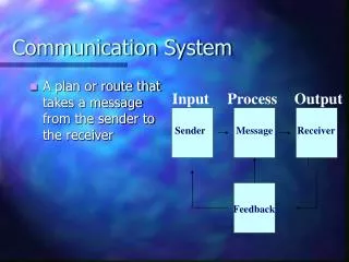
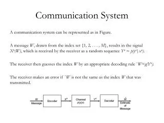
1. Communication System • A communication system can be represented as in Figure. • A message W, drawn from the index set {1, 2, . . . , M}, results in the signal Xn(W), which is received by the receiver as a random sequence Yn∼ p(yn|xn). • The receiver then guesses the index W by an appropriate decoding rule ˆW=g(Yn). • The receiver makes an error if ˆW is not the same as the index W that was transmitted.

2. Discrete Channel and its Extension • DefinitionA discrete channel, denoted by (, p(y|x), ), consists of two finite sets and and a collection of probability mass functions p(y|x), one for each x ∈ X, such that for every x and y, p(y|x) ≥ 0, and for every x, y p(y|x) = 1, with the interpretation that X is the input and Y is the output of the channel. • DefinitionThe nth extension of the discrete memoryless channel(DMC) is the channel (n, p(yn|xn),n), • where p(yk|xk, yk−1) = p(yk|xk), k = 1, 2, . . . , n.

3. Channel Without Feedback • If the channel is used without feedback • i.e., if the input symbols do not depend on the past output symbols, namely, • p(xk|x k−1, y k−1) = p(xk|x k−1), • the channel transition function for the nth extension of the discrete memoryless channel reduces to

4. (M,n) Code • An (M, n) code for the channel (, p(y|x), ) consists of the following: • 1. An index set {1, 2, . . . , M}. • 2. An encoding function Xn: {1, 2, . . .,M} → n, yielding codewords xn(1), xn(2), . . ., xn(M). The set of codewords is called the codebook. • 3. A decoding function g : n→ {1, 2, . . . , M}, • which is a deterministic rule that assigns a guess to each possible received vector.

5. Definitions • Definition(Conditional probability of error) Let • be the conditional probability of error given that index i was sent, where I (·) is the indicator function. • DefinitionThe maximal probability of error λ(n) for an (M, n) code is defined as

6. Definitions • Definition The (arithmetic) average probability of error Pe(n)for an (M, n) code is defined as • Note that if the index W is chosen according to a uniform distribution over the set {1, 2, . . . , M}, and Xn= xn(W), then by definition • Also Pe(n)≤ λ (n)

7. Definitions • Definition The rate R of an (M, n) code is • bits per transmission. • Definition A rate R is said to be achievable if there exists a sequence of ( 2nR , n) codes such that the maximal probability of error λ(n) tends to 0 as n→∞. • We write (2nR, n) codes to mean (2nR, n) codes. • DefinitionThe capacity of a channel is the supremum of all achievable rates. • Thus, rates less than capacity yield arbitrarily small probability of error for sufficiently large block lengths. Note that if C is low, this means that we need large n to decode M symbols with a low probability of error

8. Jointly Typical Sequence • Roughly speaking, we decode a channel output Y nas the ith index if the codeword Xn(i) is “jointly typical” with the received signal Yn. • DefinitionThe set A(n)of jointly typical sequences {(xn, yn)} with respect to the distribution p(x, y) is the set of n-sequences with empirical entropies -close to the true entropies: • where:

9. Jointly Typical Sequence • Theorem (Joint AEP) Let (Xn, Yn) be sequences of length n drawn i.i.d. according to • 1. Pr((Xn, Yn) ∈ A(n) ) → 1 as n→∞. • 2. |A(n)| ≤ 2 n(H(X,Y )+). • 3. If ( ˜ Xn, ˜ Yn) ∼ p(xn)p(yn) [i.e., ˜ Xn and ˜ Yn are independent with the same marginals as p(xn, yn)], then • Also, for sufficiently large n:

10. Jointly Typical Sequence • We see the proof of the 3rd part only, since the other two can be easilty proved using the AEP. • If ~Xn and ~Yn are independent but have the same marginals as Xn and Yn, then: • Where the inequality follows from the AEP: p(xn)≤ 2-n(H(X )-) because xn is a typical sequence. The same applies to yn. • With this propriety we can say that the probability that two independent sequences are jointly typical is very small for large n From 2 (|A|) H(X,Y)=H(X)+H(X|Y)

11. Jointly Typical Set • The jointly typical set is illustrated in Figure. There are about 2 nH(X)typical X sequences and about 2 nH(Y )typical Y sequences. However, since there are only 2nH(X,Y )jointly typical sequences, not all pairs of typical Xnand typical Ynare also jointly typical. • The probability that any randomly chosen pair is jointly typical is about 2−nI(X;Y). This suggests that there are about 2 nI (X;Y)distinguishable signals Xn. 2nH(Y) typical yn sequences 2nH(X,Y) jointly typical pairs (xn,yn) 2nH(X) typical xn sequences

12. Jointly Typical Set • Another way to look at this is in terms of the set of jointly typical sequences for a fixed output sequence Yn, presumably the output sequence resulting from the true input signal Xn. • For this sequence Yn, there are about 2 nH(X|Y)conditionally typical input signals. The probability that some randomly chosen (other) input signal Xnis jointly typical with Yn is about 2 nH(X|Y) /2 nH(X)= 2−nI (X;Y) . • This again suggests that we can choose about 2 nI (X;Y)codewords X n(W) before one of these codewords will get confused with the codeword that caused the output Yn.

13. Channel Coding Theorem • Theorem (Channel coding theorem) For a discrete memoryless channel, all rates below capacity C are achievable. Specifically, for every rate R < C, there exists a sequence of (2nR, n) codes with maximum probability of error λ(n) → 0. • Conversely, any sequence of (2nR, n) codes with λ(n) → 0 must have R ≤ C.

14. Channel Coding Theorem • The proof makes use of the properties of typical sequences. It is based on the following decoding rule: we decode by joint typicality; • we look for a codeword that is jointly typical with the received sequence. • If we find a unique codeword satisfying this property, we declare that word to be the transmitted codeword.

15. Channel Coding Theorem • By the properties of joint typicality, with high probability the transmitted codeword and the received sequence are jointly typical, since they are • probabilistically related. • Also, the probability that any other codeword looks jointly typical with the received sequence is 2−nI . Hence, if we have fewer then 2 nIcodewords, then with high probability there will be no other codewords that can be confused with the transmitted codeword, and the probability of error is small.

16. Proof • We prove that rates R < C are achievable: • Fix p(x). Generate a (2nR, n) code at random according to the distribution p(x). Specifically, we generate 2nRcodewords independently according to the distribution • We exhibit the 2nR codewords as the rows of a matrix: • Each entry in the matrix is generated i.i.d. according to p(x). Thus, the probability that we generate a particular code C is

17. Proof • 1. A random code C is generated according to p(x). • 2. The code C is then revealed to both sender and receiver. Both sender and receiver are also assumed to know the channel transition matrix p(y|x) for the channel. • 3. A message W is chosen according to a uniform distribution: Pr(W = w) = 2−nR, w= 1, 2, . . . , 2nR. • 4. The wth codeword Xn(w), corresponding to the wth row of C, is sent over the channel. • 5. The receiver receives a sequence Ynaccording to the distribution

18. Proof • 6. The receiver guesses which message was sent. We will use jointly typical decoding, In jointly typical decoding, the receiver declares that the index ˆW was sent if the following conditions are satisfied: • • (Xn( ˆW),Yn) is jointly typical. • • There is no other index W’ ≠ ˆW such that (Xn(W’), Yn) ∈ Aε(n). • If no such ˆW exists or if there is more than one such, an error is declared. (We may assume that the receiver outputs a dummy index such as 0 in this case.) • 7. There is a decoding error if ˆW ≠ W. Let E be the event {ˆW ≠ W}.

19. Proof: Probability of Error • We calculate the average probability of error • It does not depends on the index (because of the symmetry of code construction) • Two possible sources of error: • Yn is not jointly typical with the transmitted Xn • There is some other codeword that is jointly typical with Yn • The probability that the transmitted codeword and the received sequence are jointly typical goes to 1 (AEP). • For any rival codeword, the probability that it is jointly typical with the received sequence is approximately 2−nI • hence we can use about 2nI codewords and still have a low probability of error.

20. Proof: Probability of Error • We let W be drawn according to a uniform distribution over {1, 2, . . . , 2nR} and use jointly typical decoding ˆ W(yn) as described in step 6 • Average probability of error: • By the symmetry of the code construction, the average probability of error averaged over all codes does not depend on the particular index, then we can assume W=1 was sent. Then we have:

21. Define the following events: Ei = { (Xn(i), Yn) is in Aε(n)}, i∈ {1, 2, . . . , 2nR}, where Ei is the event that the ith codeword and Ynare jointly typical. • Recall that Ynis the result of sending the first codeword Xn(1) over the channel. • Error occurs if • Ec1 occurs (transmitted codeword and the received sequence are not jointly typical) • E2 ∪ E3 ∪ · · · ∪ E2nRoccurs (when a wrong codeword is jointly typical with the received sequence) • Hence, letting P(E) denote Pr(E|W = 1), we have • by the union of events bound for probabilities.

22. By the joint AEP, P(Ec1|W = 1)→0, and hence P(Ec1|W = 1) ≤ εfor n sufficiently large. • Xn(1) and Xn(i) are independent for i ≠ 1, then Ynand Xn(i) are independent. • the probability that Xn(i) and Ynare jointly typical is ≤ 2−n(I (X;Y)−3ε)by the joint AEP: if n is sufficiently large and R < I(X; Y) − 3ε. Hence, if R < I(X; Y), we can choose and n so that the average probability of error, averaged over codebooks and codewords, is less than 2ε.

23. Comments • Although the theorem shows that there exist good codes with arbitrarily small probability of error for long block lengths, it does not provide a way of constructing the best codes. • If we used the scheme suggested by the proof and generate a code at random with the appropriate distribution, the code constructed is likely to be good for long block lengths. • We discuss Hamming codes, the simplest of a class of algebraic error correcting codes that can correct one error in a block of bits.