Chapter 6: LSA by Computer Algebra

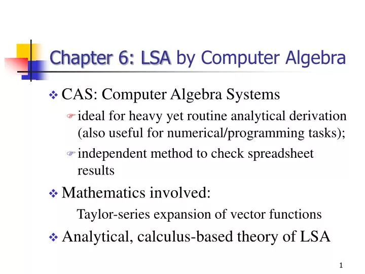
1. Chapter 6: LSA by Computer Algebra • CAS: Computer Algebra Systems • ideal for heavy yet routine analytical derivation (also useful for numerical/programming tasks); • independent method to check spreadsheet results • Mathematics involved: Taylor-series expansion of vector functions • Analytical, calculus-based theory of LSA

2. Taylor Series Expansion Taylor’s Theorem: gives approximation of f(x) at xnearx0 where x = x0 + x. Requires: (i) values of f & (various) f’, both evaluated at x0, and (ii) small quantities x: f(x)  f(x0 + x) = f(x0) + + H.O.T. (6.1) H.O.T. = “Higher Order Terms” To approximate m multi-variate functions f1(x), f2(x),…, fm(x): view collectively as components of vector function f(x), then f(x) = f(x0 + x) = f(x0) + x + H.O.T. (6.2a) Define: Aij = (6.2b)

3. Variation of Coordinates via Series Expansion Resection w/ redundant targets: measured: many (m) angles Objective: obtain the best set of (n) coordinates (i.e. E, N) for unknown station(s), that will fit the mobserved data as closely as possible. Assume: m > n. Arrange observed data into column vector:  =

4. Apply least-squares (LS) condition: • q f(x) x = LS solutionfor coordinates, e.g. x = [EU, NU]T in Section 3.5.2 (n = 2); f(x): • Computed version of measured angles or/and distances • Computed using values of the (best) coordinates x

5. Fig. 3-13 Example: f1 = calculated angle A-U-B in Fig. 3-13, where Hence f1 as a function of the unknown coordinates xis (6.4)

6. How to find the best solution x?Utilize the fact: x = x0 + x • x0 = (any) approximate solution. Thus • f(x0 + x) • Apply 6.2(a)(b):f(x0) + x + H.O.T. • Hence, x – [ – f(x0)] + H.O.T.  0 (6.5) • Note: xis the only unknown in this problem • Rephrasing (6.5): • Minimize || x – k + H.O.T. ||2 , where k – f(x0) • (weighted problem, weight matrix w) • ** If we modified a problem very slightly (dropping H.O.T.) then • the solution should only differ slightly **

7. First obtain approx. solution (really: minimizes ||Ax – k||2): x = k (6.7) • Solution improved to xnew = x0 + x (6.8) • This updated (still approximate) solution: provides a new (better) “x0“ Fig. 6.1 Improving provisional coordinates by (approximate) x • Use new x0 to repeat procedure until convergence is met

8. Calculation of derivatives (6.2b) for matrix elements Aij: • (i = 1 to m, j = 1 to n) • By hand: lengthy (m can be >> 1; n also) & error-prone • Symbolic expression to be numerically evaluated repeatedly by substituting x0; also for k= – f(x0) • Seek help from CAS tools • Maple V, Mathematica (“Mtka”), REDUCE, DERIVE, MACSYMA, MuMath, MathCAD, etc. • URL for free Mtka download (save-disallowed): • http://www.wolfram.com/products/mathematica/trial.cgi • CAS calculators

9. Resection example: • Download and install trial version of Mtka • Use program enclosed in CD-ROM • Open the file resection.mb with Mtka • Press Shift + Enter to run each line • Results should agree with Solver results in Ch. 3

10. Generic procedure • Define unknowns = x (n x 1) • Put “observed data” into q (m x 1) • Prepare computed versions of qas f(x) (m x 1) • Prepare Aij= D[fi,xj] (m x n) (symbolic) • (Reasonable) provisional solution = x0 • k= – f(x0); A -> A(x0) (numerical now) • x = (ATWA)-1ATWk • Updatex0tox0+Dx; repeat from step 6 until solution converges

11. Potential applications • Recovering missing parameters of a circle using (4 or more) observed points • Locating the center, major & minor axes of an ellipse by observed points • Parameters of a comet trajectory using observed data • Etc.