Download
1 / 24
240 likes | 409 Vues
Lecture 18. Deconvolution CLEAN Why does CLEAN work? Parallel CLEAN MEM. ‘Deconvolution’. How can we go from this to this? Deconvolution in the sky plane implies interpolation or reconstruction of missing values in the UV plane.

E N D
Lecture 18 • Deconvolution • CLEAN • Why does CLEAN work? • Parallel CLEAN • MEM
‘Deconvolution’. • How can we go from • this • to this? • Deconvolution in the sky plane implies interpolation or reconstruction of missing values in the UV plane. • But we, the human observer, can look at the top image and just ‘know’ that it is 2 point sources on a blank field.
The CLEAN algorithm. • Find the brightest pixel rb in the dirty image. • Measure its brightness D(rb). • Subtract λD(rb)B(r-rb) from the image, where λ is a number in the approximate range 0.01 to 0.2. • Repeat until satisfied. • The successive numbers λD(rb) are called clean components. Högbom J A, Astron. Astrophys. Suppl. 15, 417 (1974) Further refinements have been added by Clark and later by Cotton and Schwab, but the essential nature of the algorithm remains the same. 25/43
CLEANing Dirty image Cleaned image 26/43
CLEANing Dirty image Cleaned image 27/43
CLEANing Dirty image Cleaned image 28/43
CLEANing Dirty image Cleaned image 29/43
Problems with CLEAN: • Mathematicians don’t like CLEAN. They say it ought not to work. There are lots of papers out there proving it doesn’t. • But it does work, good enough for rough-and-ready astronomers, anyway. • This is because the real sky obeys strong constraints: • Nearly always there are just a few smallish bright patches on a blank background; • Negative flux values don’t occur in the real sky. • CLEAN doesn’t work really well on extended sources – can get ‘clean stripes’ or ‘bowl’ artifacts. • It is difficult to know when to stop CLEANing. Too soon, and you are missing flux. Too late, and you are just cleaning the noise in your image.
More problems with CLEAN: • Sources which vary in flux over the duration of the observation. • Solution: cut the observation into shorter chunks, clean separately, then recombine. • Clunky, loses sensitivity. • ‘Parallel’ cleaning works well though. • (Only relevant for wide-band case:) different sources have different shapes of spectrum. • Parallel cleaning is also good for this – even when sources vary both in frequency and time! • Sources which aren’t located at the centre of a pixel. Fixes: • Re-centre on each source, then CLEAN them away. • You guessed it – parallel cleaning can also help.
Wide-band issues:one can vastly increase the number of samples by extending the bandwidth. Simulated (e)MERLIN UV samples, δ=+35° Δf/f = 0.0005 Δf/f = 0.3 30/43
Description of the problem: an example. S f If both point sources have identical spectra, there is no problem. S f 31/43
Description of the problem: an example. More realistic: different spectra: S f S f This will not clean away. 32/43
Parallel CLEAN for wide-band observations. Conway J E, Cornwell T J & Wilkinson P N, MNRAS 246, 490 (1990) Decomposed the dirty image as a sum of convolutions. Sault R J & Wieringa M H, A&A Suppl. Ser. 108, 585 (1994) Described the parallel CLEAN algorithm. I0 I1 I2 * * * = + + … B0 B1 B2 Dirty image D 33/43
The Sault-Wieringa algorithm: νref νref νref νref ν ν ν ν • The basic idea is to construct a number of dirty beams from components of a Taylor expansion of the spectrum. 0th order S + Taylor expansion 1st order + A source spectrum: 2nd order etc…
Taylor-term beams max = 1.0 max = 0.02 max = 0.01 max = 0.004 0th order 1st order 2nd order 3rd order
A simulation to test this: 19 point sources from 0.001 to 1 Jy Spectra: cubics, with random coefficients. eg ν (GHz)
Alternate cleaning:(i) 1000 cycles of standard clean …not good.
Alternate cleaning:(ii) each spectral channel cleaned, then co-added. …pretty good, but do we lose faint sources?
S-W clean to various orders (All 1000 cycles with gain (λ) = 0.1) 0th order (equivalent to standard clean)
S-W clean to various orders 1st order
S-W clean to various orders 2nd order
S-W clean to various orders 3rd order Not much left but numerical noise.
Time-varying sources: Source constant in time Source flux varying with time
Time-varying sources: Stewart I M, Fenech D M & Muxlow T W B, in preparation. 5 sources, all ~1 Jy, varying in both flux and spectral index by ~x10. Input to the simulation (average flux; convolved with restoring beam) Dirty image Högbom clean: 2000 cycles, λ=0.1 Parallel clean: 2000 cycles, λ=0.1, Nf=3, Nt=6 All brightness scales -0.02 to +0.02 Jy