Download
1 / 33
340 likes | 508 Vues
Heat Conduction in a Body Subject to an Oscillating Heat Source. By Seth Flaxman Evanston Township High School. Problem Statement. Copper plate in contact with an oscillating heat source Tests at various velocities Measured temperature distribution Computer simulations Physical experiments.

E N D
Heat Conduction in a Body Subject to an Oscillating Heat Source By Seth Flaxman Evanston Township High School
Problem Statement • Copper plate in contact with an oscillating heat source • Tests at various velocities • Measured temperature distribution • Computer simulations • Physical experiments
Purpose • Heat conduction problems • Novel problem: oscillating heat sources at various velocities • Importance
Background Heat flow is a part of everyday life. Examples: Radiation: Heat transfer due to the sun Convection: Hot air currents in an oven Conduction: Touching something that is hot
Heat Flux Fourier’s Law of Conduction q - heat flux k - thermal conductivity T -temperature distribution, dependent on time and space
Heat Conduction Heat Equation k - thermal conductivity q - heat generation term ρ - density of the material c - heat capacity of the material T - temperature distribution
Previous Work • Work by Krishnamurthy on oscillating heat sources • Computer model developed by Backstrom A steel bar heated by a moving torch
Methods Computer Simulation and Laboratory Experiment • Copper plate • Heat source • Heat source velocity • Boundary conditions • Time period
Thermistor positions in the copper plate Laboratory Experiment
Laboratory Experiment • Each run lasted 120 seconds • Temperature readings recorded every 5 milliseconds
Computer Model • Heat equation • Boundary conditions • Insulated • Initial temperature • Heat flux Contact area in the laboratory Contact area in the computer model
Results Temperature vs. Time at 0.40 m/sec Computer Simulation Laboratory Results Temperature (ºC) Temperature (ºC) Time (sec.) Time (sec.)
Results Temperature vs. Time at 0.040 m/sec Computer Simulation Laboratory Results Temperature (ºC) Temperature (ºC) Time (sec.) Time (sec.)
Results Temperature vs. Time at 0.0079 m/sec Computer Simulation Laboratory Results Temperature (ºC) Temperature (ºC) Time (sec.) Time (sec.)
Results Temperature vs. Time at 0.0040 m/sec Computer Simulation Laboratory Results Temperature (ºC) Temperature (ºC) Time (sec.) Time (sec.)
Results Laboratory Results Temperature vs. Time at 0.40 m/sec Temperature vs. Time at 0.0040 m/sec Temperature (ºC) Temperature (ºC) Time (sec.) Time (sec.)
Laboratory Results Temperature Change by Probe (ºC)
Discussion • Interesting behavior at low velocities • Computer simulations and experimental results agree • Average rise in temperature is independent of velocity • New results, not in literature
Further Research • Analytic solution • Other types of oscillatory motion: simple harmonic motion • Slower velocities • Different materials
Acknowledgments Special thanks to Dr. Mark Vondracek, my parents, my brothers, Dr. Russell Kohnken, and Ms. Lisa Oberman. Also, thanks to David L. Vernier of Vernier Software and Technology and Marcus H. Mendenhall, author of the Python Laboratory Operations Toolkit.
Results Heat Vector Field Plot Heat Vector Field Plot (0.040 m/sec.) Location of heat source y (cm) x (cm)
Methods P = IV P = 2.12 * 10 = 21.2 W Heat flux = 21.2 / (.023 * .0275) = 33,517 W / m2 2.75 cm
Methods Heat Source Velocities (m/sec.)
FlexPDE Descriptor File TITLE 'Temperature vs. Time at 0.0040 m/sec' { intel.pde } SELECT errlim=1e-3 spectral_colors VARIABLES temp( range=400) DEFINITIONS Lx = .2286 { in meters } Ly = .1294 { in meters } RealHeight = .1524 { in meters } d0 = .0275 { length of heat source in meters } heat_flux = -33517 { W / m^2 } time_interval = 120 vx = .0040 { Moving heat source velocity in m/sec } period = (Lx - d0) / vx oscillations = time_interval / period length = Lx heat = 0 tempi = 26.5 { degrees Celsius } k = 386 {Thermal conductivity of copper } rcp= 8954 * 383.1 { Density of copper times specific heat } { Source: p. 657 of Heat Conduction Ed. 2 by Ozisik [7] } fluxd_x = -k*dx(temp) fluxd_y = -k*dy(temp) fluxd = vector(fluxd_x, fluxd_y) fluxdm = magnitude(fluxd) step = abs(ustep( mod(t, period * 2) - period) * period - mod(t, period) ) { In FlexPDE, mod does accept floats. This means repeated subtraction rather than remainder. } fluxd0 = heat_flux * [ustep(vx* step + d0 - x) - ustep(vx * step - x)] INITIAL VALUES temp = tempi EQUATIONS div(fluxd) + rcp * dt(temp) = 0 BOUNDARIES region 'domain' start (0,0) natural(temp) = 0 line to (Lx,0) natural(temp) = 0 line to (Lx,Ly) natural(temp) = fluxd0 line to (0,Ly) natural(temp)= 0 line to finish TIME from 0 to oscillations * period PLOTS for t=0 by period * .1 to oscillations * period contour( temp) painted vector( fluxd) norm elevation( fluxd0 ) from (0,0) to (Lx,0) HISTORIES HISTORY(temp) at (Lx/5,2*RealHeight/3) (2*Lx/5, 2*RealHeight/3) (3*Lx/5,2*RealHeight/3) (4*Lx/5, 2*RealHeight/3) (Lx/5,RealHeight/3) (2*Lx/5, RealHeight/3) (3*Lx/5,RealHeight/3) (4*Lx/5, RealHeight/3) END
Boundary Conditions Initial temperature (26.5 ºC): Insulated on all sides: Subject to oscillating heat flux on top: fluxd0 = heat_flux * [ustep(vx * step + d0 - x) - ustep(vx * step - x)]
Presentation Outline • Problem Statement • Purpose • Methods • Results • Further Research